Algebra Review
The math you will need to think like an economist
Here is the good news, up front: the mathematics of introductory economics is easier than almost anything you did in your last math class. There is no calculus, no trigonometry, nothing exotic. If you can handle fractions, percentages, and the equation of a line, you're going to kill it.
So why a chapter on it at all? Because in economics, math isn't the point — it's the language. A demand curve, a percentage change, the slope of a line: each is just a way of saying something about human choices more precisely than words alone can. The trouble isn't the arithmetic. The trouble is forgetting what the number means. A student who computes "elasticity = 1.8" and stops has missed the point, even if they got the right answer; the number was only ever a way to say "buyers here are quite sensitive to price."
The purpose of this chapter is to give you a refresher, some practice, and a couple of tools to help you be successful. We'll sharpen some tools, each one tied to where you'll pick it up again later, so that when the real economics starts, the math never gets in your way. Treat this as the chapter you return to whenever a later calculation feels shaky.
This is the one chapter that's a toolkit, not an argument — so it looks different: lots of worked examples and quick practice, fewer stories. Don't try to memorize it in one sitting. Work the examples, then come back whenever a later chapter's math feels uncertain. Each tool below names the chapter where you'll use it for real.
Arithmetic and Numerical Reasoning
Most economic calculations are arithmetically simple — the work is knowing which numbers to combine and what the result means. The handful you'll use most: totals (price × quantity = revenue), differences (revenue − cost = profit), and per-unit measures (a total divided by how many units).
The one habit worth building now is the per-unit instinct — taking a big total and asking "per one." It turns unlike things into comparable ones, and it's the seed of marginal thinking at the end of this chapter.
A bakery sells 200 loaves at $4 each. Its total cost for the day is $560.
- Total revenue = price × quantity = $4 × 200 = $800.
- Profit = total revenue − total cost = $800 − $560 = $240.
- Average cost = total cost ÷ quantity = $560 ÷ 200 = $2.80 per loaf.
Quick checkA stand sells 50 coffees at $3. What is total revenue?▸
Quick checkRevenue is $150 and total cost is $90. What is profit, and what is average cost over the 50 coffees?▸
Quick checkTwo factories each spend $1,000. One makes 250 units, the other 400. Which has the lower per-unit cost, and what is it?▸
Fluency target: first find the total, then the difference, then the per-unit number. In this class, you will do this anytime a problem asks about revenue, profit, average cost, or cost per unit.
- Find revenue: 80 tickets at $6 each.
- Subtract total cost of $360 to find profit.
- Divide total cost by 80 to find cost per ticket.
RevealWork the fluency target▸
Percentages and Percent Change
Economists care less about how much something changed than about how much it changed relative to where it started. A $1 price rise is trivial on a $50 textbook and enormous on a $2 coffee. The tool that captures this is percent change, and it is worth real practice now because it is the engine of the single most important calculation in the back half of this course: elasticity. We will use this repeatedly in Chapters 15 and 16.
The formula is one line: percent change = (new − old) ÷ old × 100. The only common slip is the denominator — you always divide by the starting value, not the new one. This is the most-used skill in the chapter, so the practice below is deliberately heavy.
A subscription rises from $8 to $10 per month.
- Find the absolute change: new − old = 10 − 8 = 2.
- Divide by the starting value: 2 ÷ 8 = 0.25.
- Multiply by 100: 0.25 × 100 = 25%.
Weekly sales fall from 500 units to 450. Find the percent change. The setup is filled; you finish the reasoning.
- Absolute change: 450 − 500 = −50.
- Divide by the starting value: −50 ÷ 500 = ______.
- Times 100: ______%.
Quick checkA wage rises from $20 to $23 per hour. What is the percent change?▸
Quick checkA price falls from $50 to $40. Percent change?▸
Quick check A coffee's price goes from $2 to $3. A textbook's goes from $50 to $51. Both rose by $1 — which rose more in percent terms, and roughly how much? ▸
Quick checkQuantity demanded rises 12% when price falls 6%. Ignoring the sign for a moment, divide the two percent changes (12 ÷ 6). What number do you get?▸
Retrieval practiceWhy do economists almost always prefer percent change to absolute change?▸
Because absolute change can be misleading without context, and percent change supplies that context automatically. A $1,000 raise is life-changing for someone earning $20,000 and a rounding error for someone earning $2,000,000 — the raw number is the same, but the relative change tells the real story. Percent change asks "compared to what you started with, how big was this?" — and that ratio is comparable across wildly different scales. It's also why elasticity, inflation, and growth rates are all expressed in percent: each compares a change to its own starting point.
Fluency target: name the old value, compute the change, divide by the old value, then interpret the sign. This is the move underneath inflation, growth, and elasticity.
- A price rises from $40 to $50. Find the percent change.
- A price falls from $50 to $40. Find the percent change.
- Explain why the two percentages are not opposites.
RevealWork the fluency target▸
Interactive practice 1Percent change fluency▸
Reading and Interpreting Graphs
A graph answers one question: how does one variable change when another changes? Read the axes first (what's measured, in what units), then the shape. An upward-sloping line means the two variables move together; a downward-sloping line means they move in opposite directions. Where two lines cross is a point that matters — it's where their two stories agree.
One purely visual distinction will save you all term, and we'll teach it here with no economics attached — just your eyes. There are two completely different things a graph can show:
Train your eye to tell these apart on sight. Later, in chapters 3 and 4 each will get an economic name and meaning — but the visual discrimination is a pure graph-reading skill, and it's worth owning before any economics rides on it.
Quick checkA line slopes downward. Do its two variables move together or in opposite directions?▸
Quick checkOn a graph, a dot moves to a new position but the line it sits on hasn't budged. Which of the two events is this?▸
Quick checkThe entire line lifts up and to the right. Move-along, or shift?▸
Fluency target: read the axes, describe the slope, identify what changed, and explain the graph in one complete sentence.
Interactive practice 2Read the graph first▸
Slope, Intercept, and Finding Where Lines Cross
Most intro models use straight lines, because a line is fully described by two numbers: where it starts (the intercept) and how steeply it climbs or falls (the slope). Written out, any line is:Y = intercept + slope × X
Slope is rise over run — the change in the vertical variable divided by the change in the horizontal. A positive slope rises; a negative slope falls. It is the single most useful number on any graph, because it answers "if X changes by one, how much does Y change?"
A relationship is written Q = 100 − 2P.
- Match it to Y = intercept + slope × X, with Q as Y and P as X.
- The intercept is 100 — when P = 0, Q = 100.
- The slope is −2 — each one-unit rise in P lowers Q by 2.
- Check a point: at P = 10, Q = 100 − 2(10) = 80.
Now the move you'll use most: finding where two lines cross. Two lines intersect at the one point where their values are equal — so to find it, you set the two equations equal to each other and solve for the shared value. This single technique, mechanical here, becomes the way you find a market's equilibrium the moment two curves enter the same graph in chapter 3.
Two lines: Y = 2 + X and Y = 10 − X. Find where they cross.
- At the crossing, both lines have the same Y at the same X — so set the right-hand sides equal: 2 + X = 10 − X.
- Collect the X terms on one side: X + X = 10 − 2, so 2X = 8.
- Solve: X = 4.
- Put X = 4 back into either equation to get Y: Y = 2 + 4 = 6 (check: 10 − 4 = 6 ✓).
Quick checkFor Y = 5 + 3X, what are the slope and intercept?▸
Quick checkA line passes through (0, 10) and (5, 0). What is its slope?▸
Quick checkFind where Y = 1 + 2X and Y = 13 − X cross.▸
Quick checkTwo lines cross at (3, 7). If you plug X = 3 into both equations, what must you get?▸
Retrieval practiceWhy does setting two equations equal to each other find their intersection?▸
Because the intersection is, by definition, the one point that lies on both lines at once — the single X where the two lines produce the same Y. Setting the equations equal says exactly that: "find the X at which line A's Y equals line B's Y." Solve it and you have the shared X; substitute back to get the shared Y. Every other point fails the test, because away from the crossing the two lines give different Y-values for the same X. When you meet this again in Chapter 3, the two lines will be supply and demand, the shared X will be the equilibrium quantity, and the shared Y will be the equilibrium price — but the algebra is identical to what you just did.
Fluency target: plug into a line, read its slope, then set two lines equal when you need the crossing point.
- For Y = 2 + 3X, find Y when X = 4.
- Name the slope and explain it in words.
- Find where Y = 2 + 3X crosses Y = 14 - X.
RevealWork the fluency target▸
Technology and Math
A graphing calculator is not a substitute for understanding the algebra, but it is a powerful fluency tool. Use desmos.com/calculator when you want to see a line, check an intersection, or make sure your table and equation tell the same story. In my class, desmos' calculator is always allowed for use on everything except proctored quizzes and exams.
The basic workflow is simple: enter one equation per line, usexfor the horizontal variable andyfor the vertical variable, then click the crossing point to read its coordinates. If your economics equation is written with P and Q, translate it first: price usually behaves like one axis and quantity like the other. The graph is a check on your thinking, not a magic answer machine.
Suppose two lines are Y = 2 + 3X and Y = 14 - X.
- Open Desmos and type
y = 2 + 3xon the first line. - On the second line, type
y = 14 - x - Click the crossing point to read the coordinates.
- Use the algebra to verify: 2 + 3X = 14 - X, so X = 3 and Y = 11.
Fluency target: use Desmos to see the lines, but still prove the answer with algebra. The tool should make you faster and more confident, not more dependent.
- Enter
y = 10 - 2x - Enter
y = 1 + x - Click the crossing point, then verify it by setting the equations equal.
RevealWork the fluency target▸
Triangles and Rectangles: The Size of a Region
Here's a fact that surprises people: some of the most important quantities in economics aren't points or lines on a graph — they're areas. The value buyers get from a market, the value sellers get, the value destroyed by a bad policy, a firm's total revenue, the money a tax raises — each of these is the size of a region you read off a supply-and-demand diagram. So you need to be able to measure two shapes, and the good news is you already learned both in middle school.
A rectangle's area is just:base × heightWhen a firm sells 200 loaves at $4 each, its total revenue is a rectangle — 200 wide, $4 tall — with area $800. A triangle's area is half of that:½ × base × heightThat single formula is the workhorse: nearly every "value created" or "value destroyed" region in this course is a triangle, and you'll compute its area again and again(we'll do this a lot in chapter 6).
The only skill beyond the formula is reading the base and height off the axes. The base is the region's width — usually a quantity, measured along the horizontal axis. The height is its vertical extent — usually a price or a gap between two prices, measured up the vertical axis. Get those two numbers and the area falls right out.
A triangle sits against the axes: it runs from a quantity of 0 to 30 along the bottom, and its height drops from $90 down to $50 — a vertical gap of $40 — over that span.
- Identify the base — the horizontal width: 30 (a quantity).
- Identify the height — the vertical gap: 90 − 50 = 40 (a price difference).
- Apply the formula: area = ½ × base × height = ½ × 30 × 40.
- Compute: ½ × 1200 = 600.
Quick checkA triangle has base 20 and height 15. What's its area?▸
Quick checkA rectangle is 50 wide and 8 tall (think: 50 units sold at $8). What's its area?▸
Quick checkA triangle's base runs from a quantity of 10 to 40, and its height is the gap between $70 and $55. Find the area.▸
Retrieval practiceWhen you read a triangle off a supply-and-demand graph, what do the base and height usually represent?▸
The base is almost always a quantity — a width measured along the horizontal axis (how many units the region spans). The height is almost always a price or a gap between two prices — a vertical distance up the price axis. So a surplus or deadweight-loss triangle multiplies "how many units" by "how big a price gap" and halves it. The single most common mistake is forgetting the ½ (which would give a rectangle's area instead) or mixing up which axis gives the base — base is the horizontal quantity, height is the vertical price. Keep "base = quantity, height = price gap, then halve" in mind and the surplus and deadweight-loss computations in Chapter 6 are pure plug-in.
Fluency target: identify whether the region is a rectangle or triangle, find the base and height from the graph, then attach the economic meaning.
- A rectangle is 30 units wide and $8 tall.
- A triangle has base 30 and height $8.
- Say which one might represent total revenue and which one might represent surplus or deadweight loss.
RevealWork the fluency target▸
The Rule of Four
Here is the habit that, more than any single calculation, marks someone who understands economics: the ability to take one relationship and move freely among words, a table, a graph, and an equation. Each form reveals something the others hide. A table gives you exact numbers; a graph shows the shape at a glance; an equation lets you compute any point; words tell you what it all means. Someone who can only work in one form is pattern-matching. Someone who can translate among all four genuinely understands.
This is so central that we built a box for it, and you'll see it return in nearly every chapter from here on. Watch one simple demand relationship take all four shapes at once:
The same relationship, Q = 100 − 2P, expressed every way economists use. Learn to slide among these and the rest of the course gets dramatically easier:
Q = 100 − 2PThe 100 is the intercept; the −2 is the slope. Plug in any price, get the quantity.A table shows: P = 0 → Q = 60; P = 10 → Q = 40; P = 20 → Q = 20. Find the equation.
- The intercept is the Q when P = 0: that's 60.
- The slope is rise over run: from P = 0 to P = 10, Q falls 60 → 40, a change of −20 over +10, so slope = −20 ÷ 10 = −2.
- Assemble Y = intercept + slope × X form: Q = 60 − 2P.
- Check the last row: at P = 20, Q = 60 − 2(20) = 20 ✓.
Quick checkIn words, what does Q = 50 − 5P say about how price and quantity relate?▸
Quick checkA table reads P = 0 → Q = 30; P = 5 → Q = 20; P = 10 → Q = 10. What's the equation?▸
Quick checkFor Q = 100 − 2P, what quantity goes with a price of 25?▸
Fluency target: take one idea through words, equation, table, and graph. That is the real skill, not memorizing one format.
- Words: as price rises, quantity demanded falls by 3 units per $1.
- Equation: quantity is 90 when price is zero.
- Make the equation and compute Q when P = 10 and P = 20.
RevealWork the fluency target▸
Interactive practice 3Rule of Four translation▸
Thinking at the Margin
The last tool is less a calculation than a way of seeing, and it is the bridge into the whole course. Most real decisions aren't all-or-nothing — they're about one more. Not "should a bakery exist?" but "should it bake one more loaf?" Not "is studying good?" but "is one more hour worth it tonight?" The economist's word for "one more" is marginal, and the central rule of the entire subject fits in a sentence: do something as long as its marginal benefit exceeds its marginal cost, and stop when they meet.
The key is to separate marginal from total and from average. Total is everything so far; average is the total spread evenly over the units; marginal is just the next one. Decisions live at the margin because the past is already spent — what you control is the next step.
A food truck can make one more taco for an added cost of $1.50 (extra ingredients, time). It would sell for $4.
- Marginal cost of the next taco = $1.50.
- Marginal benefit (the revenue it brings) = $4.
- Compare: $4 > $1.50, so the next taco adds more than it costs.
Quick checkThe next unit costs $6 to make and would sell for $5. Make it?▸
Quick checkYou've studied 3 hours (total). A 4th hour would raise your grade a little but cost you needed sleep. What kind of comparison decides whether to do it?▸
Quick checkA factory's total cost for 10 units is $100; for 11 units it's $108. What is the marginal cost of the 11th unit?▸
Retrieval practiceWhy do economists focus on the margin instead of the total?▸
Because decisions are about what to do next, and only marginal quantities answer that. The total tells you where you've been; the average smooths over the individual steps; but the choice in front of you is always "one more or not?" — and that's settled by comparing the benefit and cost of that single next unit. Focusing on totals leads to classic errors, like refusing to abandon a failing project because of all you've already spent (the past total is gone; only the next step is a real choice). The whole course will return to this: firms produce until marginal cost meets marginal revenue, consumers buy until marginal benefit meets price. Master "compare the next one" now and the logic of the entire subject is already in your hands.
Fluency target: ignore totals when the question is about one more. Compare marginal benefit to marginal cost, decide, then say why.
- You have already studied 3 hours.
- A 4th hour would raise your score by 4 points but cost you sleep worth 6 points to you.
- Should you study the 4th hour?
RevealWork the fluency target▸