Supply and Demand II:
Shifts, Shocks, and Price Controls
First, do no harm
The date: June 17, 1971. The speaker: Richard M. Nixon, President of the United States of America. The occasion: a briefing for the public about a new concern and priority for the US government.
President Nixon said, "America's public enemy number one in the United States is drug abuse. In order to fight and defeat this enemy, it is necessary to wage a new, all-out offensive."
With those words, the war on drugs was born.
The last chapter gave us tools for snapshots: supply and demand at one moment in time. On that basis, the strategy looked simple: squelch supply by punishing suppliers with fines, prison, and sometimes death. And on its own terms, it worked. Kingpins were killed or captured one after another: Pablo Escobar, shot dead on a Medellín rooftop in 1993; the Cali bosses; then dozens of Mexican capos.
So here is the puzzle.
In the short run the price of cocaine jumped, just as you'd expect when supply is cut. That was the point: at higher prices, fewer people would buy.
And then, over the long run, through decades of seizures and fallen kingpins, the drug on American streets did not get scarcer or dearer. Adjusted for purity, it fell to a fraction of where it began. Choke the supply, and the drug got cheaper.
Meanwhile a very different intervention was failing in a very different way. A city, watching rents climb, does the humane and obvious thing: it caps them, so that no landlord may charge more than $1,000 for a one-bedroom. A year on, the tenants who kept their apartments pay less — and everyone else is worse off. Apartments vanish. Waiting lists stretch for years.
To understand either story, a snapshot isn't enough; we need to compare. This chapter finishes the list of what moves supply and demand curves, then turns to comparative statics: what happens to the equilibrium price and quantity when a curve shifts. Then we follow a price that is free to move, as it pulls new sellers into a market, and a price that isn't, as a cap freezes a shortage in place. By the end, both puzzles have the same answer: the price kept doing its job, and the policies didn't expect it to.
Related Goods and Income Effects
Imagine for a moment that your demand for hot dogs is constant, but hot dog buns suddenly become prohibitively expensive. While your willingness to buy hot dogs hasn't changed, your ability to buy hot dogs has. In other words, demand is affected by things other than the good itself. The price of one good can shift the demand for another. Which way depends on how the two goods are related.
Keep the own-price test in mind here. Suppose ride-share prices jump for the new "Myft" service. What will happen to Qd? It will decrease. What has happened to demand? So far, nothing. In the ride-share market, riders move along the demand curve: that's the good's own price. But what about the bus market? Those switching from "Myft" to buses consider them close substitutes, so demand shifts right.
To help you build intuition, it can be helpful to use the perfect version of a substitute or a complement. Imagine a substitute that is so perfect that you cannot even tell the difference between two goods. Some examples include certain nuts, bolts, and washers, and other basic hardware tools. If a perfect substitute becomes cheaper, most people will switch without hesitation. If the substitute suddenly becomes more expensive, meanwhile, demand for the original good will go up. While perfect substitutes are rare in practice, the logic holds even with imperfect substitutes.
Similarly, imagine a right-shoe left-shoe market. (In most places, we sell complements in pairs, but it's a useful way to build your thinking patterns.) If left shoes skyrocket in price, you will buy fewer right shoes because together they are more expensive. Similarly, if left shoes plummet in price, you will buy more because you can afford more pairs. That logic holds when things are imperfect complements.
Income Effects
When we say that demand is about being willing and able, one of the simplest ways to expand the ability to pay for more goods is an increase in income. Those who win the lottery have more ability to buy goods than those who have not. And most goods follow the rule: the more money you have, the more you spend on those goods: food, housing, clothing, and so on. We call these normal goods, which are goods that you buy more of as you grow richer.
Next we have the kind of good you buy less of when you get richer: an inferior good — instant noodles, the cross-town bus. These are goods you can finally afford to skip in favor of the nicer option. Note: inferior does not have anything to do with quality; it's simply a measure of what people choose to buy as they get wealthier.
Taxes, Subsidies, and Shocks
On the supply side, let's take a look at how government policy can affect producers. A tax on each unit sold works like a higher cost: sellers need a higher price to offer the same quantity, so supply shifts left. A subsidy works the other way and shifts supply right.
Taxes and subsidies are just a narrow part of a bigger web of possible effects that can jolt an economy. The triggering event itself — the frost, the lumber spike, the new employer downtown — is a called a shock: a sudden, often unexpected change in one of these underlying forces. A supply shock changes costs or the number of sellers; a demand shock jolts buyers. Keep the two words straight: the shock is the event out in the world, the shift is what it does to the curve on the page.
And now the case from the hook. When enforcement jails suppliers, seizes shipments, and raises the risk of dealing, fewer sellers are willing to supply at any given price. Nothing about buyers changed, and the drug's own price didn't do the moving — the whole supply curve slid left. Interdiction is a supply shock, and the next concept reads what it does.
| Force that changes | Shifts demand… | Shifts supply… |
|---|---|---|
| Income rises (normal good) | right | — |
| Income rises (inferior good) | left | — |
| Price of a substitute rises | right | — |
| Price of a complement rises | left | — |
| Tastes shift toward the good | right | — |
| Buyers expect a higher price soon | right | — |
| Number of buyers rises | right | — |
| Input cost rises | — | left |
| Better technology | — | right |
| Tax on the good | — | left |
| Subsidy for the good | — | right |
| Sellers expect a higher price soon | — | left (hold back now) |
| Number of sellers rises | — | right |
Quick checkA popular streaming show makes a neighborhood famous. What happens to the demand curve for apartments there, and which way?▸
Quick checkThe city doubles the property tax on rental buildings. Shift or movement along — and which curve, which way?▸
Quick checkPrinters get much cheaper. What happens to the demand for ink cartridges?▸
Quick checkYour income rises, and you stop buying store-brand ramen. For you, is ramen normal or inferior, and which way does your demand for it shift?▸
One caution before we move on: everything above is about what shifts a demand curve. A different question is whether demand always slopes the usual way — less bought as price rises. Almost always, yes. But two famous oddballs break it, and they're too fun to skip.
A Veblen good is wanted because it's expensive: a $30,000 watch, a handbag whose whole point is the price tag. Cut the price and you can kill the appeal — so demand can rise with price. (Named for Thorstein Veblen's "conspicuous consumption.") A Giffen good is rarer and stranger: a cheap staple so central to a poor household's budget that when its price rises, the household is now too poor to afford the pricier foods it used to mix in — so it buys more of the staple. The textbook cases are potatoes or rice for the very poor, though clean real-world Giffen goods are nearly impossible to pin down, and economists still argue over the few candidates. You could imagine rice next to costly meat such that when the price of rice goes up, the family buys more precisely because they can no longer afford meat.
While the ideas behind Veblen and Giffen goods are interesting, you should treat both as curiosities — we flag them so the rule's exceptions don't ambush you, not because they'll be on the exam. What's more, they are very hard to identify in real life. Rather, they are evidence that economists know that their models have limits, and a good economist is willing to investigate just how far their assumptions will hold.
Retrieval practiceGive a headline that would shift the supply of apartments left, and one that would shift demand right. Name the shifter in each.▸
Many answers work. Supply left: "Lumber and labor costs surge" (input costs) or "City adds new building fees" (tax). Demand right: "Tech firm relocates 5,000 jobs downtown" (number of buyers) or "Incomes climb after a boom" (income, normal good). The test is always the same: is the cause something other than the apartment's own rent? If yes, it's a shift, and you only need to decide which curve and which direction. Naming the wrong curve is the usual slip — a tax falls on sellers, so it moves supply, even though buyers feel the resulting price.
Comparative statics
One of the simplest and most useful aspects to introductory economics is building an intuition around price and quantity. Knowing a curve shifted is half the job. The other half is predicting what happens to equilibrium price and quantity once a curve has shifted. Economists call this comparative statics. We'll do it on the same apartment market from Chapter 3 (equilibrium $1,200, 300 units), so you should have some familiarity with this market.
We'll begin with one curve moving.
In this example, we'll use the drug market. To keep the arithmetic clean, say a unit trades at $100, and buyers take 100 units. The government introduces significant enforcement measures, leading suppliers to leave the market out of fear, capture, or death. Supply shifts left. Demand for an addictive drug is steep: heavy users cut back only a little when the price rises. (A later chapter gives that steepness a name: elasticity.) Suppose the new supply crosses demand at $150 and 90 units.
- Supply shifts left: at every price, fewer sellers. The crossing climbs the demand curve to a higher price.
- Price: $100 → $150 (up 50%). Quantity: 100 → 90 (down only 10%, because demand is steep).
- Now the sting. Revenue is price × quantity. Before: $100 × 100 = $10,000. After: $150 × 90 =$13,500.
A large firm opens downtown, adding renters at every rent. Demand shifts right; suppose quantity demanded rises by 200 at every price, so the new demand is Qd= 1100 − 0.5P. Supply is unchanged at Qs= −300 + 0.5P.
- Set new quantity demanded equal to quantity supplied: 1100 − 0.5P = −300 + 0.5P.
- Collect terms: 1100 + 300 = P, so 1400 = P.
- New equilibrium rent: P = $1,400 (up from $1,200).
- Substitute back: Q = −300 + 0.5(1400) = 400 (up from 300).
A modular-building method lowers costs, so landlords supply 200 more at every rent: Qs = −100 + 0.5P. Demand is back to its original Qd = 900 − 0.5P.
- Set equal: 900 − 0.5P = −100 + 0.5P.
- Collect: 900 + 100 = P, so P = $1,000.
- Your turn: substitute to find the new quantity.
- Your turn: which way did rent and quantity move, and how does that compare with the employer example?
AnswerReveal steps 3 and 4▸
Quick checkRemote work lets renters leave town, and demand shifts left. Supply doesn't change. What happens to rent and quantity?▸
Quick checkSolo: supply shifts left (lumber prices spike). Which way do rent and quantity move?▸
The post-shift market (demand right to Qd= 1100 − 0.5P, supply unchanged) described four ways. Each form is the same function — the numbers reconcile across all four, and every form lands on the equilibrium $1,400, 400.
Qs= −300 + 0.5P
P* = 1400 Q* = 400
| P | Qd | Qs |
|---|---|---|
| 1000 | 600 | 200 |
| 1200 | 500 | 300 |
| 1400 | 400 | 400 |
Now the harder, and more interesting, case: both curves shift at once. This happens constantly in the real world — the employer arrives and construction gets cheaper in the same year. The surprise is that when both move, you can usually pin down only one of price and quantity for certain. The other is indeterminate— its direction depends on which shift is bigger, which the model alone doesn't tell you.
Take both shifting right — more renters and more units. Quantity clearly rises (both forces push it up). But rent? The demand increase pushes rent up; the supply increase pushes it down. Try to predict rent and quantity yourself before opening the example.
Both curves move right — what happens to rent and quantity?▸
Demand right by 200 (Qd= 1100 − 0.5P)andsupply right by 200 (Qs= −100 + 0.5P) — equal-sized shifts.
- Set equal: 1100 − 0.5P = −100 + 0.5P.
- Collect: 1100 + 100 = P, so 1200 = P.
- Rent is unchanged at $1,200 — the two pressures exactly cancel.
- Substitute: Q = −100 + 0.5(1200) = 500 (up from 300).
The easiest way to get this down is to build a table enough times that it becomes automatic. There are rules that can help, but the simplest way I know of is to draw graphs and build intuitions.
Here are two example rules. When the two curves move the same way, quantity is pinned down and price is ambiguous. When they move opposite ways, price is pinned down and quantity is ambiguous.
If those work for you, great. But if not, draw a simple S & D graph, then move one of the two curves. Note what happens to price and quantity, then rinse and repeat until the full table is filled in. You'll notice that when both supply and demand shift outward the quantity is guaranteed to spike, but we can't be sure of the price: if supply goes up a lot and demand up only a little, then price will drop. If supply goes up a little and demand goes up a lot, you'll still have a little price spike.
| Supply ↑ (right) | Supply unchanged | Supply ↓ (left) | |
|---|---|---|---|
| Demand ↑ (right) | Q↑ ·P ? | P↑, Q↑ | P↑ ·Q ? |
| Demand unchanged | P↓, Q↑ | no change | P↑, Q↓ |
| Demand ↓ (left) | P↓ ·Q ? | P↓, Q↓ | Q↓ ·P ? |
The middle row and middle column are the single shifts — one curve moves, the other holds still — and there both price and quantity are always determinate. The four corners are the double shifts.
With a precise estimate, we could tell exactly what Q and P would be, of course. We only use the term indeterminate because we don't have such a clear estimate. Note: "indeterminate" is stronger than "we didn't bother": the model depends on things the diagram alone doesn't fix — chiefly the relative sizes of the two shifts, and secondarily how steep the curves are. Some shifts can even leave things even.
Interactive practice 1Predict the new equilibrium▸
Quick checkDemand rises and supply falls at the same time (more buyers, costlier to build). Which is determinate — price or quantity?▸
Quick checkYou observe that quantity definitely rose but the price change is ambiguous. What kind of double shift happened?▸
Quick checkBoth curves shiftleft. What can you say about price and quantity?▸
Retrieval practiceWithout looking, rebuild the rule: when is price determinate, and when is quantity?▸
Same-direction shifts (both right or both left) →quantityis determinate, price ambiguous. Opposite-direction shifts (one right, one left) →priceis determinate, quantity ambiguous. The intuition: when both forces push quantity the same way, quantity can't be in doubt — but they tug price in opposite directions, so price is the casualty. Flip it for opposite shifts. The single most common error is trying to pin downbothvariables; with a double shift, one of them is genuinely unknowable from the model alone, and saying so is the correct answer, not a cop-out.
Entry and Exit
One of the unexpected rules of economics is that over time, economic profits will end up at zero. We will explore this at significant depth later, but for now it's worth mentioning the mechanism. If a price is also an incentive, let's see what happens when that price works over time. A high equilibrium price doesn't just ration what's already for sale; it tells everyone who could sell that there's money to be made, and some of them come. Economists call that entry. A low price does the reverse: sellers who can't cover their costs mothball units, switch lines, or leave. That's exit.
Entry takes time. A new builder needs permits and a year of construction; a new drug route needs contacts and couriers. So economists separate the short run, before anyone new can arrive, from the long run, after entry and exit have played out. (Entry and exit return as the engine of long-run competition, where they grind profit down to zero in later chapters.)
When new sellers arrive, apply Chapter 3's test. At the old price, is a different quantity offered than before? Yes: there are more sellers now, so more is offered at every price. That's a shift of supply to the right, even though the high price is what attracted them. The price is the reason sellers came; the number of sellers is what changed.
Compare the landlords already in a city who list a few more units when rent rises. Nobody new arrived; existing sellers responded to the price. That's a movement along supply.
Pick up the interdiction example from Concept 2 and let time run.
- Before. The market clears at $100 a unit, 100 units (E0).
- Short run. Interdiction shifts supply left. The price climbs to $150 and quantity falls to 90 (E1). Sellers' revenue rises from $10,000 to $13,500.
- Long run. That bigger prize is a recruitment poster. New suppliers and new routes enter, and supply shifts back to the right. Other forces pushed the same way over those decades (smuggling got more efficient, production expanded), so supply ended up to the right of where it started.
- New equilibrium. The price settles at $60 and quantity at 108 (E2): cheaper and more plentiful than before the crackdown.
But watch what the model does not price, in the spirit of the unseen cost from Chapter 1. Entry here is not a peaceful queue of new shopkeepers. When a kingpin is removed, the territory he held does not stay orderly; it fragments, and the fragments fight to inherit it. By one count the number of major organized-crime groups in Mexico rose from roughly five in 2006 to around sixty by 2012, and studies of the "kingpin strategy" find that removing a leader sharply raises the odds his organization splinters — with a spike in killings to follow. The seen result was an arrest. The unseen result was a war, and a supply chain that barely flinched. That gap between the seen and the unseen is the whole cost of reading a market by its intentions instead of its incentives.
None of this says enforcement is pointless or that the model settles what policy should be — the historical verdict is genuinely contested, and the market's answer to a supply shock is a positive fact, not a normative recommendation. What the model does say, cleanly, is what to expect: cut the supply of a good with steep demand and the short-run price rises, the revenue rises, and the long-run answer is entry.
Quick checkA new ski resort draws crowds, and nightly rents for condos near it soar. Over the next five years, what happens to the supply of short-term rentals nearby, and why?▸
Quick checkStreaming wipes out the video-rental business, and prices for rentals collapse. What happens to the number of stores, and which curve moves?▸
Quick checkWhen rent rises, the landlords already in a city list a few more units. Entry, or a movement along supply?▸
Retrieval practiceIn two sentences: what does interdiction do to a drug's price in the short run, and why can the long run look so different?▸
In the short run, interdiction shifts supply left, so the price rises (and with steep demand, sellers' revenue rises too). In the long run, that high price attracts entry, which shifts supply back to the right, and the price can end up lower than where it started. A wrong answer stops at the short run, or calls entry a movement along the curve: the new sellers change the number of sellers, so supply shifts.
Price controls
The drug market swallowed its shock: cut its supply and, given time, the high price pulled entry in until the price sank back and then below. That rescue depended on the price being free to move. Now take that freedom away. A price ceiling is a law forbidding any price above some level. Rent control is the classic case. The intuition behind it is humane: rents are too high, so cap them. But recall what Chapter 3 built: a price is a signal, and a shortage cures itself only because the price is free to rise toward equilibrium. A binding ceiling forbids exactly that rise. So the shortage it creates cannot self-correct. It is permanent.
First, a crucial distinction: a ceiling only does something if it's set below the equilibrium price. A ceiling above equilibrium — say, a $1,400 cap on a market that clears at $1,200 — is non-binding: the market never wanted to go that high, so nothing changes. The cap bites only when set below where the market would clear.
Again, let's use an intuition. Imagine a $2 minimum wage, or perhaps a consumer-protection bill that sets pencils maximum price at $4000. Neither do anything, so the economic impact is nil. Why do politicians still pass such things? Sometimes, for the virtue signaling; sometimes, an out-of-date minimum wage simply hasn't kept up to speed with inflation. In any case, the key idea here is simple: it's only "binding" if it makes a difference.
Our market clears at $1,200 (300 units). The city caps rent at $1,000. Using the Chapter 3 schedules: at $1,000, Qd= 900 − 0.5(1000) = 400 and Qs= −300 + 0.5(1000) = 200.
- At the $1,000 ceiling, renters want 400 apartments but landlords offer only 200.
- Shortage = 400 − 200 = 200 apartments.
- In a free market this shortage would bid rent up toward $1,200, erasing itself. The ceiling forbids any rent above $1,000.
- So the price can't rise, the 200 missing units never appear, and the shortage stays — month after month.
If price can't ration the 200 scarce apartments, something else must. That something is non-price rationing, and it is never pretty: years-long waiting lists, apartments passed through personal connections, landlords letting buildings decay because demand far exceeds supply anyway, under-the-table "key money," and black markets. The 1970s gave a vivid cousin of this — when gasoline prices were capped, the shortage showed up as hours-long lines and stations simply running dry.
Step back for the deeper lesson, because it outlasts apartments. A scarce thing will be rationed — that part is not optional. You can ration by price, by queue, by lottery, or by who-you-know, but ration you must, because there isn't enough to go around. Capping the price doesn't abolish the rationing; it only changes the currency you pay in — from dollars to hours in line, favors, and luck. And price has one power none of its replacements share: because it is also an incentive, it doesn't merely decide who gets today's apartments — it pays builders to make more of them tomorrow. A waiting list rations the shortage and freezes it there; a free price rations it and goes to work erasing it. That is the quiet cost of breaking the thermometer.

The mirror image is a price floor — a legal minimum. It binds only when set above equilibrium, and then it produces a persistent surplus instead of a shortage. Agricultural price supports are the textbook case: set a floor under the price of milk above what the market would pay, and you get year-after-year mountains of unsold dairy the government must buy up or store. The most famous floor of all is the minimum wage — a floor under the price of labor — but its effects are genuinely debated and we give it its own chapter.
Note, too, that both the political left and right hate price controls. Sometimes. Similarly, both the left and right believe that there are worthy exceptions to the no-price-controls rules. The political left prefers to protect consumers with price ceilings; the political right prefers to protect sellers with price floors.
Another intuition builder: ceiling ought to be high. Floors ought to be low. But when a floor is unnaturally high, the result will be distortion; similarly, a ceiling that is too low will result in problems. When you see a graph of a price floor that is set low, it will not bind anything. Only a high price floor carries distortionary effects in the form of surplusses. Similarly, when you see a ceiling that is high, you needn't worry about it too much. But when a ceiling is low enough to interfere with supply and demand, be ready for shortages.
Quick checkA city caps rent at $1,300 in a market that clears at $1,200. A year later, a big employer arrives and the market would clear at $1,400. Binding then? Binding now?▸
Quick checkThe rent ceiling is lowered from $1,000 to $800. Using the Ch 3 schedules, what's the new shortage?▸
Quick checkA price floor on milk is setbelowthe equilibrium price. Binding or not?▸
Interactive practice 2Binding or not?▸
Common misconception"A price ceiling makes apartments cheaper for everyone."▸
It makes them cheaper for the people whoalready have one— and unavailable for everyone still searching. At the $1,000 cap, only 200 apartments are supplied where 400 are wanted; 200 would-be renters who'd happily pay get nothing at all. For them the price didn't fall, it became infinite.
And the lucky 200 don't escape free either. The "true price" they pay re-emerges in forms money can't measure: months on a waiting list, an apartment that never gets repaired, a finder's fee paid in cash, a landlord who rents only to friends. Add up the waiting and the side payments and the decay, and the real cost of a rent-controlled apartment oftenexceedswhat the market rent would have been.
A widely cited study of San Francisco's 1994 expansion of rent control (Diamond et al., 2019) found the policy did what the model predicts on both sides. Tenants in covered units were substantially more likely to stay put — real protection, the intended effect. But landlords responded by converting and redeveloping to escape the rules,reducingthe supply of rental housing by around 15% — which pushed market rentsupcitywide for everyone outside the controlled units.
The honest reading: rent control is not a free lunch and not a pure villain either. It transfers real benefits to incumbent tenants while shrinking supply and raising rents for newcomers — exactly the "who pays the scarcity, and in what form" question above. Whether that trade is worth making is a values question, not a settled one, and economists who agree on themechanismstill disagree on thepolicy. That disagreement is where the readings and policy prompt pick up — it is not something the model alone can resolve.
The moves you can now make
Three questions at the level the exam will actually ask — application, not recall. Try each on paper first, then reveal the worked solution. The trying is where the learning happens.
Type A · single shift & comparative statics
The government adds a new tax on every pound of coffee sold. Identify which curve shifts and in which direction, then state what happens to the equilibrium price and quantity of coffee, and explain why.
Show worked solution▸
The tax raises the cost of selling each pound of coffee, so it shifts thesupplycurveleft— not demand, and not a slide along supply, because the trigger isn't coffee's own price.
A leftward supply shift moves the equilibrium up the unchanged demand curve: pricerisesand quantityfalls. Intuition: less is available at every price, so buyers bid the price up, and at the higher price fewer cups are bought. The tell that it's a supply story, not a demand story, is that price and quantity move inoppositedirections.
Type B · double shift & indeterminacy
In the smartphone market, consumer incomes rise (phones are a normal good) and at the same time a manufacturing breakthrough lowers production costs. Predict the effect on equilibrium price and quantity. If either is indeterminate, say so and explain why.
Show worked solution▸
Higher incomes shift demandright; the cheaper process shifts supplyright. Both curves move thesamedirection.
Quantity isdeterminate: both forces push it up, so equilibrium quantity rises. Price isindeterminate: the demand increase pushes price up while the supply increase pushes it down, and which wins depends on the relative sizes of the two shifts — which the model alone doesn't give us. The correct, full-credit answer names quantity as rising and states explicitly that price cannot be pinned down without knowing which shift is larger. Trying to call price anyway is the classic error.
Type C · price controls
A campus textbook market is described by the equations below, and clears at a price of $80 with a quantity of500books:
- • Demand: Qd= 1100 − 7.5P
- • Supply: Qs= −100 + 7.5P
A student government, calling prices unfair, caps the price at the $60 shown above. Determine whether the cap is binding, compute the resulting shortage, and name one form of non-price rationing likely to appear.
Show worked solution▸
- The cap ($60) isbelowthe equilibrium price ($80), so it isbinding— it forces the price below where the market would clear.
- Quantity demanded at $60: Qd= 1100 − 7.5(60) = 1100 − 450 = 650.
- Quantity supplied at $60: Qs= −100 + 7.5(60) = −100 + 450 = 350.
- Shortage = Qd− Qs= 650 − 350 = 300 textbooks.
Put the moves together
A coastal city's market for one-bedroom apartments is initially in equilibrium. Then a large technology firm relocates 5,000 employees downtown. Alarmed by rising rents, the city council responds with a rent ceiling.
- Draw a correctly labeled supply-and-demand graph for apartments, showing the initial equilibrium rent (R1) and quantity (Q1).(2 pts)
- Show the effect of the firm's relocation on your graph, and state what happens to the equilibrium rent and quantity.(2 pts)
- Suppose after the relocation demand is Qd= 1100 − 0.5R and supply is Qs= −300 + 0.5R. Calculate the new equilibrium rent and quantity. Show your work.(2 pts)
- The council caps rent at $1,000. On your graph, show the ceiling and identify the resulting shortage. Is the ceiling binding? Explain.(3 pts)
- Identify one form of non-price rationing likely to emerge under the ceiling.(1 pt)
Reveal a full-credit response▸
(a)A standard graph: vertical axis Rent ($), horizontal axis Quantity of apartments, downward-sloping D and upward-sloping S crossing at E1, with R1dropped to the price axis and Q1to the quantity axis. (See figure.)
(b)The relocation adds buyers, sodemand shifts rightto D′. Equilibrium rentrises(R1→R2) and equilibrium quantityrises(Q1→Q2). Both move up because a demand increase slides the crossing up the unchanged supply curve.
(c)Set Qd= Qs: 1100 − 0.5R = −300 + 0.5R → 1400 = R → R = $1,400. Substitute: Q = −300 + 0.5(1400) =400.
(d)The $1,000 ceiling is drawn as a horizontal line below E′ ($1,400). At $1,000, Qd= 1100 − 0.5(1000) = 600 and Qs= −300 + 0.5(1000) = 200, a shortage of 400 (the horizontal gap between S and D′ at the ceiling). The ceilingis bindingbecause it is set below the equilibrium rent of $1,400 — it forces rent under where the market would clear, so the price can't rise to erase the shortage.
(e)Any one of: waiting lists/queues, landlord favoritism, deterioration of unmaintained units, "key money" side payments, or a black market in leases.
Reveal the scoring rubric▸
- 1 pt(a) Axes labeled (Rent on vertical, Quantity on horizontal) with a downward D and upward S.
- 1 pt(a) Initial equilibrium marked where D and S cross, with R1and Q1indicated.
- 1 pt(b) Demand shown shiftingright(a new curve D′, not a movement along D).
- 1 pt(b) States both equilibrium rent AND quantityrise.
- 1 pt(c) Correct equilibrium rent R = $1,400 with work shown (Qdset equal to Qs).
- 1 pt(c) Correct equilibrium quantity Q = 400.
- 1 pt(d) Ceiling drawn as a horizontal linebelowthe new equilibrium.
- 1 pt(d) Shortage identified as the gap between Qsand Qdat the ceiling (here 400, or shown on the graph).
- 1 pt(d) States the ceiling is binding AND explains it is below equilibrium.
- 1 pt(e) Names a valid form of non-price rationing.
Ten independent points — each earned on its own, the way a real reader scores it. A wrong number in (c) doesn't cost you the (d) points if your shortage logic is right given your own equilibrium.
Reveal what loses points▸
- ConceptualIn (b), drawing amovement alongdemand instead of a rightwardshift— the Chapter 3 trap. A relocation changes the number of buyers, which moves the whole curve, not a point on it.
- PrecisionIn (c), writing the answer "$1,400" with no equation set up. AP "Calculate" prompts require shown work; a correct number with no work routinely earns nothing.
- Exam craftIn (d), saying "the ceiling causes a shortage" without stating it isbinding because it is below equilibrium. The "Explain" verb wants the mechanism, not just the outcome — and an unlabeled ceiling line (no value, no horizontal placement) forfeits the graph point even when the prose is right.
Interfere with a market — by any of many means — and you push it off the equilibrium that was coordinating it. Sometimes the market absorbs the blow, as the drug trade did through entry; sometimes a pinned price forbids it to, and the distortion gets a whole lot worse.
they'd treat a price as information before treating it as a target — because a supply shock, a cap, a tax, a quota all push a market off equilibrium, and the distortion is often not the one intended. Drugs, gas, and rent are three of many cases; the chapters ahead measure and catalogue the rest.
- Every intervention moves a market off equilibrium and pays for it in distortion; a binding ceiling makes a lasting shortage, a floor a lasting surplus, and a supply shock a price the market then unwinds through entry.
- Rent control protects today's tenants — at the cost of less housing and higher rents for everyone else.
- Is protecting today's tenants worth shrinking tomorrow's housing?
- Distortion is not the same as "bad": some are worth their cost. That is Chapter 3's rule — override a price only with a reason — and Chapter 6 puts a number on the cost so the reason can be weighed.
If you're not paying for something in money, ask what you're paying for it in.
If you have a line, you likely aren't charging enough.