Welfare Analysis
Also, the deadweight loss of Christmas
Christmas, it turns out, is the problem.
You spend $50 on a sweater for your cousin. He smiles, says thanks, and quietly finds a way to return it. Between the drive, the line, and the store credit he'll never quite use, the sweater ends up worth about $30 to him. Let's pause on this: $50 of resources went in, $30 of value came out, and $20 simply… evaporated. Not stolen, not transferred to anyone — just gone. No one is $20 richer for it. The world is poorer by twenty dollars and a sweater nobody quite wanted.
In 1993 an economist named Joel Waldfogel did the arithmetic on this for the whole holiday season and published it under the magnificently grumpy title "The Deadweight Loss of Christmas." He surveyed his Yale students about the gifts they'd just received — what the giver had paid, and what each gift was actually worth to them. His finding: holiday gifts destroy somewhere between a tenth and a third of their value. With Americans spending about $40 billion on holiday gifts at the time, that came to something like $4 billion to $13 billion of value vanishing every December. Waldfogel later stretched the idea into a whole book, Scroogenomics, where he describes the season as an exercise in "value destruction." Bah, humbug, with a statistical regression.
This is a Scrooge-ish way to open a chapter, but it points at something profound and genuinely useful: economists can measure the value a trade creates, in dollars, off a supply-and-demand graph. Last chapter you watched trade create value but could only describe it; this chapter hands you the ruler. And once you can measure the value created, you can measure the value destroyed when the right trades don't happen — by a clumsy gift, a price control, a tax, a monopoly. That measurement is the payoff of everything in Unit 1. It's how we put a number on "markets create value," and on what it costs when they're blocked.
Consumer and Producer Surplus
When you get a great deal at the store, say, you buy a nice backpack for $5 on clearance that you would have paid $50 for, you receive $45 in consumer surplus. When you get a great college job that pays way above the market rate, say, $25 per hour when you would have insisted on at least $15, you get $10 an hour of producer surplus. Last chapter we learned about the gains from trade, which we could only describe. Now, we see that they can be measured — in dollars, right off a supply-and-demand graph. This is the power of markets, quantified.
Most of economics asks what will happen — where the price lands, how much gets traded, etc. This is a different kind: it asks how good an outcome is for the people living in it, and whether some other outcome might be better. Welcome to a branch of the discipline called welfare economics. A warning about the word, because it trips up almost everyone. In everyday American speech, "welfare" means public assistance — a government check. Here it means something older and broader: well-being, how well a person's life is going. A welfare analysis isn't a study of welfare programs. It's an accounting of how much better off a market leaves the people in it — and how much worse off when the market is blocked.
In the last chapter, "gains from trade" came from specialization — Crusoe fishing, Friday gathering, each doing what they sacrifice least to make. Ch 5But value is also created whenever a buyer and seller simply exchange, with no specializing at all: if you'd happily pay $90 for a thing and I'd let it go for $45, the trade manufactures value out of the gap between us. These are two engines — gains from specialization and gains from exchange — and they are not rivals; they compound. You specialize to make a thing at low cost, then exchange it with someone who values it more than you do, and value is created at both steps. The tool we build now measures both, and we can use a simple supply and demand curve to measure it. What we're looking for is the wedge between what a unit is worth to a buyer and what it costs a seller.
Remember back to chapter 2: each point on a demand curve is somebody's willingness to pay — the marginal value of that unit to that buyer. The curve slopes down because, one buyer to the next and one unit to the next, that value falls. So the demand curve is a ranked list of what each unit is worth to the people who want it.
Now suppose the market price is $60 and you'd have happily paid $90. You buy, hand over $60, and walk away with $30 of value you didn't have to pay for. That $30 is your consumer surplus— the value you captured beyond what you spent. Add up that gap for every buyer in the market and you get total consumer surplus: on the graph, it's the area below the demand curve and above the price.
Sellers have a mirror-image story. The supply curve is each seller's willingness to accept— the least they'd take, which is their cost of making that unit. A seller who'd have sold for $45 but receives $60 keeps $15 of producer surplus. Summed across sellers, that's the area above the supply curve and below the price. Put the two together — consumer surplus plus producer surplus — and you have total surplus: the entire value the market created by letting these trades happen.
Using the anchor market — demand P = 100 − 2Q, supply P = 40 + Q, equilibrium at P = $60, Q = 20 — find consumer and producer surplus.
- Each surplus is a right triangle, so use area = ½ × base × height. The base is the equilibrium quantity, 20.
- Consumer surplus height = (demand's price-intercept) − (price) = 100 − 60 = 40. So CS = ½ × 20 × 40 = $400.
- Producer surplus height = (price) − (supply's price-intercept) = 60 − 40 = 20. So PS = ½ × 20 × 20 = $200.
- Total surplus = CS + PS = 400 + 200 = $600.
Those triangles are no classroom abstractions. They are real measures of how much better off you are, in economic terms, from specialization and trade; and some of them are simply enormous. Try this: what does Google cost you? Nothing — the price is zero. On the graph, that means your consumer surplus is the entire area under your demand curve. In a 2019 study, the economists Erik Brynjolfsson, Avinash Collis, and Felix Eggers set out to measure it by flipping the question around. Instead of asking what people would pay for search, they asked how much people would have to be paid to give up every search engine for a year. The median answer was $17,530. Email came in around $8,400; digital maps around $3,600. None of that shows up in GDP, which counts what people spend, not what they get. It shows up only as surplus — a quiet, enormous gap between what these services cost and what they're worth.
Consumer surplus is hard to measure because you need the whole demand curve. Uber's surge pricing offered a rare opening: when demand spikes, fares jump by set multiples, so nearly identical trips are offered at many prices and you can watch who still books. Using almost 50 million ride sessions from four big U.S. cities, a team that included Steven Levitt (of Freakonomics) estimated that UberX created about $6.8 billion of consumer surplus nationwide in 2015 — roughly $1.60 for every dollar riders spent. (Two of the five authors worked for Uber, which supplied the data.)
Quick checkA buyer would pay $25 for a concert ticket and gets in for $18. What's their consumer surplus?▸
Quick checkSolo: A market clears at P = $50, Q = 30. The demand price-intercept is $110. What is consumer surplus?▸
Quick checkSolo: Same market (P = $50, Q = 30). The supply price-intercept is $20. Find producer surplus and total surplus.▸
Retrieval practiceWhy is the demand curve the right tool for measuring the value buyers get — and how does Chapter 2 explain its shape?▸
Because the height of the demand curve at each quantity is a buyer's willingness to pay — the marginal value of that unit, which Chapter 2 showed is marginal utility in dollars. Ch 2So the gap between the curve and the price is, unit by unit, value received minus value paid: the buyer's surplus. The curve slopes down because of diminishing marginal utility, which is why the surplus triangle narrows toward equilibrium. The common mistake is confusing willingness to pay with the price paid; surplus is exactly the gap between them.
Efficiency
The equilibrium quantity maximizes total surplus — exactly, not approximately. Every unit a buyer values above its cost (demand above supply) creates surplus, and at the market price it trades. Every unit beyond that would cost more to make than anyone will pay, and at the market price it doesn't. Produce less and you leave good trades on the table; produce more and you force bad ones.
Economists love (like love love) efficiency. We have a bunch of different kinds. They're all lovely. Three are worth keeping straight:
That a competitive equilibrium passes the allocative and Pareto tests at once is important enough to be called a theorem: the First Fundamental Theorem of Welfare Economics, or just the First Welfare Theorem. A competitive market equilibrium is Pareto efficient. Nobody plans it; each person watches only the price and their own situation. It's the gains from trade of Ch 5and the spontaneous order of Ch 3with a dollar figure attached: Adam Smith's invisible hand, weighed and counted.
If that sounds too good to be true, Vernon Smith agreed. As a Harvard graduate student he had watched a classroom market run by his professor, Edward Chamberlin, in which prices wandered all over the place. So in 1956, on the first day of his own class at Purdue, Smith tried again. He gave each student a secret card — buyers a maximum they could pay, sellers a minimum they could accept — and let them call out bids and offers across the room, round after round. No one knew the curves but Smith. He expected a mess. Instead, prices closed in on the equilibrium he had drawn, and the class captured nearly all the possible gains from trade. The result survived decades of variations, and in 2002 it helped earn him a Nobel Prize.
The theorem does have fine print. It holds only when:
When a condition fails, the efficiency of the market collapses. Much of the second half of this course is a tour of those failures. The best-known critiques of markets — Arthur Pigou's on spillovers, Joseph Stiglitz's on hidden information — are claims that the fine print fails, not that the theorem is wrong.
Efficiency, in any of its senses, is only about the size of the pie. It says nothing about whether the people who get the surplus deserve it, need it, or already have plenty. A market that efficiently allocates life-saving medicine to whoever can pay maximizes total surplus while a poorer, sicker person goes without; an allocation in which one person holds nearly everything can still be Pareto efficient. Economists lean on efficiency anyway because a bigger pie means everyone could be better off — but "could" is doing heavy lifting. How the pie is divided —equity— is partly a question of values no surplus calculation can settle. Is this efficient? and is this fair? are different questions, and a serious answer needs both. Ch 18Ch 20
Note that the economist's language fails us a bit here. When a layperson hears an economist blathering on about "efficiency," they naturally think: Do they even care about regular human well-being, or just cold corporate profits? But notice the pivot: in welfare economics, efficiency is human flourishing. When an economy achieves allocative and productive efficiency, it isn't just optimizing a spreadsheet; it is liberating people from the crushing friction of poverty. Look at the alternative—price controls and distorted markets that create empty shelves, endless rationing lines, and wasted human potential. By contrast, the systems that reliably generate economic efficiency are the same ones that give people the security, health, and freedom to pursue meaningful work, raise families, and actually flourish.
Now, let us return to the equity and efficiency debate. If efficiency is so important, is it always at odds with equitable distribution? Yes, allocatively efficient markets will also be Pareto efficient, and that's pretty cool. But you could still live in a world of haves and have-nots, rich trillionaires and those eking out a life under crushing poverty.
The Second Fundamental Theorem of Welfare Economics gives us a possible bridge between efficiency and equity. Any Pareto-efficient outcome — including one far more equal than the market happens to produce — can be reached through a competitive market; but rather than playing games with prices that lead to devastating distortions, the best path is redistribution at the start. Consider a one-time tax on rich to poor: you can still achieve efficiency under such a scheme. You don't have to shrink the pie to slice it differently: change who owns what, and leave the prices alone.
The second theorem also has assumptions, however. The theorem assumes behavior-agnostic lump-sum transfers, but redistribution tends to change behavior. Real taxes and benefits always change something — how much people work, how much they earn — so real redistribution carries some deadweight loss of its own. We can't quite say that "fairness is free." But we might be able to say "there is usually a more effective way to pursue fairness than freezing a price." The second welfare theorem suggests that maybe the best way to solve poverty is to simply give people money, which we'll take up as a potential policy at the end of the chapter.
Quick checkA market produces fewer units than the equilibrium quantity. Is total surplus larger or smaller than at equilibrium, and why?▸
Quick checkIn one sentence each: what does the First Welfare Theorem say, and what does the Second add?▸
Quick checkA chemical plant dumps waste into a river that a town downstream drinks from. Which condition of the First Welfare Theorem fails?▸
Quick check"This outcome is efficient, so it must be fair." What's wrong with that sentence?▸
Retrieval practiceWhy do economists put so much weight on efficiency if it ignores fairness entirely?▸
Because a bigger total surplus means more value exists to share — an efficient outcome makes it possible for everyone to be better off, even if it doesn't guarantee it. Inefficiency destroys value that no one gets, which is hard to defend on any grounds. So efficiency is a sensible first screen: are we wasting value? But it deliberately brackets who ends up with the surplus, and that question — equity — depends on values a calculation can't supply. The Second Welfare Theorem is the bridge: it says the two questions can often be handled separately, redistributing first and letting prices work second.
Deadweight Loss
If the equilibrium quantity maximizes total surplus, then anything that pushes the market away from it must shrink the pie. The lost surplus has a name: deadweight loss— value that disappears, captured by no one. This is the crucial difference from a simple transfer. When a tax moves $10 from your pocket to the government's, that's a transfer: you lose, they gain, the surplus still exists somewhere. Deadweight loss is worse — it's surplus that stops existing at all, because the trade that would have created it never happens.
Picture our anchor market with something holding the quantity at 10 instead of the efficient 20. Every unit between 10 and 20 was a trade where the buyer valued the good more than it cost to make — a trade that should have happened and created surplus. Block them, and that surplus is simply gone. It shows up on the graph as a triangle between the demand and supply curves, from the restricted quantity out to the efficient one. (In the next concept we'll see that "something holding the quantity at 10" is, concretely, a price control.)
The anchor market (demand P = 100 − 2Q, supply P = 40 + Q, efficient Q = 20) is restricted to Q = 10. Find the deadweight loss. (Note: this is far easier to do by graphing. Go to Desmos.com/calculator. Put in the two equations and manipulate them to solve.)
- Find the gap between willingness to pay and cost at the restricted quantity. At Q = 10: demand price = 100 − 2(10) = 80; supply price = 40 + 10 = 50.
- That vertical gap is the triangle's height: 80 − 50 = 30.
- The base is the quantity of lost trades — from the restricted 10 out to the efficient 20: 20 − 10 = 10.
- Deadweight loss = ½ × base × height = ½ × 10 × 30 = $150.
Quick checkSolo: A market's efficient quantity is 50. A regulation holds it at 35. At Q = 35, willingness to pay is $40 and marginal cost is $22. Find the deadweight loss.▸
Quick checkWhy is deadweight loss worse than a tax that simply transfers money from buyers to the government?▸
Quick checkBack to the hook: you pay $50 for a gift your cousin values at $30. Where's the deadweight loss, and why did it happen?▸
Think back to the beginning of the chapter: that clumsy Christmas gift that someone wants to return? It is deadweight loss in a Santa hat: a "trade" where the giver guesses wrong about the recipient's willingness to pay, so value is destroyed. The fix is the one Chapter 2 implied — let people choose for themselves, because no one knows your marginal utility better than you. Waldfogel's surveys bear this out. Gifts from partners and parents, who know your tastes, lost roughly a tenth of their value; gifts from aunts, uncles, and grandparents lost about a third. And the relatives who know you least turn out to be the likeliest to hand over cash or a gift card. Grandparents, it seems, are intuitive economists. Cash isn't unromantic; it's efficient.
The deadweight loss of Christmas is real, but giving everyone money at Christmas is, unfortunately, still frowned upon. Ask me how I know.
Price Controls
Begin with a question the last three concepts now let us answer in a sharper way: what happens when the price is simply wrong? Suppose it sits above the equilibrium — too high. Sellers, tempted by the high price, want to sell more than buyers want to buy; unsold units pile up as excess supply (often just called a surplus — a word we'll untangle below). Or suppose it sits below equilibrium — too low. Buyers want more than sellers will provide, and a shortage (excess demand) opens. We met the mechanics of both back in Chapter 3. Ch 3What we can add now is the welfare reading: a price away from equilibrium isn't just out of balance — it's inefficient. Value-creating trades are going unmade, total surplus sits below its maximum, and a deadweight-loss triangle has opened.
In a free market, none of this lasts. Excess supply has sellers shading their prices down to move stock; a shortage has buyers bidding the price up. The price slides back to the crossing, the triangle closes, and efficiency is restored — that was Chapter 3's lesson, now with a welfare price tag. Disequilibrium is a force, not a resting place. So the inefficiency of a "wrong" price is, in a free market, temporary: the market corrects itself.
Unless it can't. A price controlis a law that forbids the price from moving — and it is precisely the case where the inefficiency does not self-correct. It is held open, by force of law, indefinitely. There are two kinds, mirror images of each other:
Either way, the controlled price stops the two quantities from meeting, and one side ends up rationed. The rule for how much actually trades is simple and worth memorizing: the short side wins. Whichever quantity is smaller at the controlled price — what sellers will supply under a ceiling, or what buyers will buy under a floor — is the amount that actually changes hands. Because that amount is always below the efficient quantity, a binding control always destroys surplus. The unmade trades between the controlled quantity and the efficient one are a deadweight-loss triangle, exactly the one from the last concept — only now we know its cause has a name.
Anyone who drove in America in the 1970s has seen this diagram come to life. Price controls on oil and gasoline — an outgrowth of President Nixon's 1971 freeze on wages and prices — held the price at the pump below what the market would have set. When oil supplies tightened in 1973 and again in 1979, the price wasn't allowed to rise and ration the gas, so something else did the rationing: the line. Drivers waited for hours, some arriving before dawn. Several states let you buy only on odd or even days, depending on the last digit of your license plate. The remaining controls were lifted in early 1981, and the nationwide gas lines of that decade never returned.
Anchor market (demand P = 100 − 2Q, supply P = 40 + Q, equilibrium $60/20). The government sets a price ceiling of $50. Find the quantity traded, the shortage, and the deadweight loss.
- Is it binding? $50 is below the $60 equilibrium, so yes — it bites.
- Quantity supplied at $50 (from supply): 50 = 40 + Q → Qs= 10. Quantity demanded at $50 (from demand): 50 = 100 − 2Q → Qd= 25.
- Shortage = Qd− Qs= 25 − 10 = 15. The short side (sellers) wins, so only 10 units actually trade.
- Deadweight loss: at the traded quantity 10, demand price = 80, supply price = 50, so height = 30; base = efficient 20 − traded 10 = 10. DWL = ½ × 10 × 30 = $150.
Same $50 ceiling. Compare consumer and producer surplus before and after — Fig 6.1 against Fig 6.3.
- Before the ceiling (Fig 6.1): CS = $400, PS = $200, total = $600.
- Producer surplus after: the triangle above supply and below $50, out to the 10 units that trade. Height = 50 − 40 = 10; base = 10. PS = ½ × 10 × 10 = $50.
- Consumer surplus after: the area below demand and above $50, out to 10 units. It's a trapezoid — height 100 − 50 = 50 at Q = 0 and 80 − 50 = 30 at Q = 10. CS = 10 × (50 + 30) ÷ 2 = $400. (Or split it: a triangle ½ × 10 × 20 = $100 sitting on a rectangle 10 × 30 = $300.)
- Check the books: CS + PS + DWL = 400 + 50 + 150 = $600. Same total as before, now split three ways instead of two.
Common misconception"A price floor creates a surplus — and surplus is the good stuff."▸
Economists use the word "surplus" for two unrelated things, and this chapter uses both. Consumer and producer surplus are values— dollars of benefit, the good stuff that total surplus adds up. A surplus in the sense of excess supply is a quantity— unsold units piling up because the price is too high. The two have nothing to do with each other. In fact, the floor that creates the pile of unsold goods shrinks total surplus, as Fig 6.4 shows.
To keep them straight, this book says "excess supply" for the pile and saves "surplus" for value. Other books and exams won't always be so careful, so read the context: "a surplus of 15 units" is a quantity; "consumer surplus of $225" is a value.
Same market. Now a price floor of $70 (think an agricultural support price). The mechanical setup is filled; you finish the deadweight loss.
- Binding? $70 is above the $60 equilibrium → yes, it bites, and creates excess supply.
- At $70: quantity demanded 70 = 100 − 2Q → Qd= 15; quantity supplied 70 = 40 + Q → Qs= 30. Excess supply = 30 − 15 = 15.
- Short side now is buyers (15), so 15 units trade. Height at Q = 15: demand price 70 − supply price 55 = 15. Base = 20 − 15 = 5.
If the gas line is what a binding ceiling looks like, a cheese cave is what a binding floor looks like. For decades the U.S. government propped up milk prices with a floor, and it enforced the floor the only way a floor can really be enforced: by promising to buy whatever farmers couldn't sell at the support price. Farmers responded exactly as the supply curve predicts — they produced more — and the government bought the difference, turning it into cheese, butter, and powdered milk that could be stored. By 1981 it owned more than 560 million pounds of cheese, over two pounds for every American, much of it stacked in underground caves in Missouri and Kansas. Storing all that dairy cost around a million dollars a day, and some of it was going moldy. That December, President Reagan began giving it away: the five-pound blocks of "government cheese" that a generation of low-income families still remembers.
Notice what the cheese does to our triangle. The diagram assumes only the 15 units buyers want get produced. But when the government stands ready to buy the excess, farmers produce all 30 — so society pays the full cost of 15 extra units nobody wanted at that price, and then pays again to store them. The $37.50 triangle is a floor's minimum cost. A floor backed by government purchases costs far more.
Quick checkSolo: Under the $70 floor (Fig 6.4), find consumer surplus and producer surplus. Who gains and who loses compared with equilibrium?▸
Quick checkA city sets a rent ceiling above the current market rent. What happens?▸
Quick checkUnder a binding price ceiling, which side determines how much actually trades — buyers or sellers?▸
Quick checkSolo: Demand P = 120 − 2Q, supply P = 30 + Q (equilibrium P = $60, Q = 30). A price ceiling of $45 is imposed. Find the quantity traded and the deadweight loss.▸
Because efficiency was never the only goal. Price controls are almost always reached for on equity grounds: to protect tenants from rising rents, farmers from collapsing prices, workers from low wages. Whether that fairness gain is worth the deadweight loss turns on values a triangle can't supply. But the Second Welfare Theorem adds a pointed question: if the goal is to help renters, why not give them purchasing power and let rents clear? Part of the answer is political. A price control costs the government nothing on paper — the bill is paid by landlords, and by would-be renters who never find an apartment.
Two caveats. The model assumes competitive markets; where a single dominant employer sets wages, a floor can behave differently, which is why the minimum wage remains a genuine empirical dispute rather than a settled diagram. Ch 17Ch 18And a shortage still gets rationed — by queues, waiting lists, falling quality, favoritism, black markets — and those burn real resources, so the true cost of a binding ceiling is often larger than the triangle alone.
Common misconception"A price ceiling on rent helps tenants — it makes housing cheaper."▸
It helps some tenants — the ones who already hold a rent-controlled lease now pay less. But at the capped price, landlords supply fewer units (converting to condos, not building, letting quality slide) while more renters want in, so a chronic shortage opens. The evidence matches the diagram. When San Francisco extended rent control to small apartment buildings in 1994, landlords of the newly covered buildings cut the rental housing they offered by 15 percent, which pushed rents up about 5 percent across the rest of the city (Diamond, McQuade & Qian). Tenants already inside were protected; renters who arrived later paid more.
So the honest verdict is mixed. Rent control transfers surplus from landlords to incumbent tenants — arguably the point — while shrinking the housing supply and destroying value through shortage. And as the worked example showed, buyers as a group may gain nothing at all. A ceiling doesn't make housing cheaper for everyone; it makes housing scarcer, and cheaper only for whoever's already inside.
Retrieval practiceWhy does every binding price control create deadweight loss — ceiling or floor, no exceptions?▸
Because both push the quantity actually traded below the efficient quantity. A binding ceiling sits below equilibrium, so sellers supply less; a binding floor sits above equilibrium, so buyers buy less; either way the short side rules and fewer units change hands than at the crossing. The trades that vanish — between the controlled quantity and the efficient one — are all value-creating: the buyer valued the unit above the seller's cost. That surplus is destroyed, captured by no one, which is the definition of deadweight loss. The control may also transfer surplus between buyers and sellers (that's the redistribution it's usually after), but the shrunken quantity guarantees a triangle of pure loss on top of any transfer. The only way a control avoids deadweight loss is to be non-binding — i.e., to do nothing at all. Ch 4
Can we solve poverty with cash?
Should we simply give cash to the poor? Everything in this chapter bears on the answer. Surplus measures what help is actually worth to the person receiving it. The Second Welfare Theorem says you can redistribute without freezing prices. Price controls showed what happens when you try to help by forcing a price to stand still. The economist's instinct leans toward cash. But the case for in-kind help is stronger than it first looks.
- Recipients know their own needs best. A dollar of cash is worth at least a dollar to them; a dollar of groceries may be worth less — the sweater problem.
- It leaves prices free to coordinate, so it opens no deadweight-loss triangle in the market it touches.
- The "they'll spend it on vices" worry mostly doesn't hold up: a review of 19 studies, mostly in lower-income countries, found cash transfers didn't raise spending on alcohol or tobacco (Evans & Popova).
- In-kind aid is often cash in disguise anyway. This is known as fungibility: most SNAP households already spend more on food than their benefit, so the benefit frees up money for other things (Hoynes & Schanzenbach).
- One check is simpler to run than dozens of programs, each with its own rules and staff.
- It targets itself. Help you have to go get — a food order, a work assignment — is less attractive to people who don't really need it (Nichols & Zeckhauser).
- Society may care about specific outcomes: that children eat and families are housed, not just that budgets are bigger.
- Taxpayers are often more willing to fund food than cash, so in-kind programs may mean more total help.
- Cash has side effects too. In a recent U.S. experiment paying $1,000 a month for three years, recipients worked 1 to 2 fewer hours a week and earned about $1,900 a year less (Vivalt and colleagues).
- Help that comes with a relationship — someone who knows the family — can build self-reliance in a way a check can't.
Many readers of this book know one in-kind system from the inside. The welfare program of The Church of Jesus Christ of Latter-day Saints is built on the in-kind side of this table by design. Its handbook asks bishops to avoid giving cash when possible, to provide groceries and services through bishops' orders, to pay bills directly to the provider rather than to the member, and to invite those who receive help to work or serve as they are able. The logic is targeting and relationship: a bishop knows the family, the help is shaped to what they actually need, and the goal is self-reliance rather than dependence. It's a thoughtful answer to the same question economists argue about — and a reminder that where you land depends partly on evidence and partly on what you think help is for.
If you side with cash, what would a cash-first system look like? In 1962 Milton Friedman — the century's most famous champion of free markets — proposed an answer in Capitalism and Freedom: a negative income tax. Pick an income threshold. Earn above it and you pay tax, as now. Earn below it and the tax runs in reverse: the government pays you a fraction of the gap. No storehouses, no vouchers, no price held still by law — just cash, scaled to need, delivered through the tax system.
Friedman's pitch was that it could replace much of the patchwork of programs that had grown up one at a time. Fig 6.5 is one attempt to draw that patchwork.

Two features make Friedman's design clever. Because you keep part of every extra dollar you earn, it never fully punishes work, the way programs that cut benefits off at a hard line can. No more welfare cliff. And because it runs through the tax system, it needs little new bureaucracy. The idea came remarkably close to law: in 1969 President Nixon proposed a version, the Family Assistance Plan, which passed the House and died in the Senate. Its closest descendant is the Earned Income Tax Credit, created in 1975 and now one of the largest antipoverty programs in the country. Federal experiments with the full idea in the 1970s found what the in-kind side would predict: recipients worked somewhat less — modestly for primary earners, more for second earners and teenagers. Friedman explains the idea himself in a short clip linked in Learn More.
With the principle, overwhelmingly. In a classic survey of American economists (Alston, Kearl & Vaughan, 1992 — the figures Gregory Mankiw's principles textbook reports), 84 percent agreed that cash payments raise recipients' welfare more than in-kind transfers of equal value, and 79 percent agreed the welfare system should be restructured along the lines of a negative income tax. (Rent control fared worse: 93 percent agreed a ceiling on rents reduces the quantity and quality of housing.)
But that doesn't mean that economists are on board with a radical reform. In 2016 the Clark Center asked a panel of leading economists whether a $13,000-a-year basic income for every adult, paid for by eliminating all transfer programs — Social Security and Medicare included — would beat the status quo. One agreed, 7 were uncertain, and 26 disagreed. Their worry wasn't cash; it was scrapping targeted help for the people who need the most. The details, in other words, are where the devil lives. (The 1990s survey is also old enough that a new one could shift the numbers.)
So: the sweater, or the cash? For your cousin, the economics is easy — cash, or at least a gift card. For a society, it's harder, and this chapter has given you the tools to see why. Economics can tell you that cash usually delivers more well-being per dollar, that price controls destroy surplus, and roughly what each design costs. It can't tell you how much help a society owes, or whether help should come with conditions and a relationship attached. Those are questions for citizens.
Quick checkEconomists overwhelmingly favor cash over in-kind aid of equal value, yet most rejected a $13,000 basic income that replaced every program. Is that a contradiction?▸
The moves you can now make
Four questions at the level the exam will actually ask — surplus as areas, the deadweight loss of a control, and the efficiency-versus-equity read. Try each on paper first, then reveal the worked solution. The trying is where the learning happens.
Type A · consumer, producer, and total surplus
A market has demand P = 80 − Q and supply P = 20 + 2Q. Find the equilibrium price and quantity, then compute consumer surplus, producer surplus, and total surplus. Show your work.
Show worked solution▸
- Equilibrium: set demand = supply. 80 − Q = 20 + 2Q → 60 = 3Q → Q = 20, and P = 80 − 20 = $60.
- Consumer surplus = area below demand, above price: height = (demand intercept) − price = 80 − 60 = 20; base = 20. CS = ½ × 20 × 20 = $200.
- Producer surplus = area above supply, below price: height = price − (supply intercept) = 60 − 20 = 40; base = 20. PS = ½ × 20 × 40 = $400.
Type B · binding price ceiling & deadweight loss
A market is described by demand P = 90 − Q and supply P = 30 + 2Q, clearing at $70 and 20 units (shown below). The government imposes a price ceiling of $50. Determine whether it is binding, find the quantity that actually trades and the size of the shortage, and compute the deadweight loss.
Show worked solution▸
- The ceiling ($50) is below the equilibrium price ($70), so it is binding — it forces the price under where the market clears.
- Quantity supplied at $50 (from supply): 50 = 30 + 2Q → Qs = 10. Quantity demanded at $50 (from demand): 50 = 90 − Q → Qd = 40.
- Shortage = Qd − Qs = 40 − 10 = 30. The short side (sellers) wins, so only 10 units trade.
- Deadweight loss: at the traded quantity 10, demand price = 90 − 10 = 80 and supply price = 30 + 2(10) = 50, so height = 30; base = efficient 20 − traded 10 = 10. DWL = ½ × 10 × 30 = $150.
Type C · the mirror — a binding price floor
A market has demand P = 60 − Q and supply P = 20 + Q (equilibrium $40, 20 units). A price floor of $50 is imposed — think a minimum wage or a crop support. Find the quantity traded, the amount of excess supply, and the deadweight loss.
Show worked solution▸
- Binding? $50 is above the $40 equilibrium → yes, it bites, and creates excess supply.
- At $50: quantity demanded 50 = 60 − Q → Qd = 10; quantity supplied 50 = 20 + Q → Qs = 30. Excess supply = 30 − 10 = 20.
- Now the short side is buyers (10), so only 10 units trade.
- Deadweight loss: at Q = 10, demand price = 60 − 10 = 50 and supply price = 20 + 10 = 30, so height = 20; base = efficient 20 − traded 10 = 10. DWL = ½ × 10 × 20 = $100.
Type D · efficiency, equity, and what's a transfer
A city caps apartment rents below the market level. (i) Name one group that gains and one that loses. (ii) Of the surplus the cap removes, explain the difference between the part that is merely transferred and the part that is deadweight loss. (iii) Can this outcome be both inefficient and, to some people, fair? Explain why those are two separate questions.
Show worked solution▸
(i) Gains: the tenants who manage to get a rent-controlled unit (they pay less than before). Losses: landlords (lower rent received), and the would-be renters who can't find a unit at all once the shortage opens.
(ii) The lower price moves some surplus from landlords to the tenants who still rent — that is a transfer; the value still exists, just in different hands. The deadweight loss is different: it is the surplus from apartments that are now never rented or never built (the trades between the reduced quantity and the efficient one). That value is destroyed outright — no one captures it.
(iii) Yes. "Inefficient" is a positive claim — total surplus is below its maximum, which the diagram shows. "Fair" is a normative claim about how the remaining surplus is distributed — someone who weighs protecting incumbent tenants heavily may judge the redistribution worth the lost efficiency. Efficiency is about the size of the pie; fairness is about the slicing. A complete answer needs both, and economics settles only the first.
Put the moves together
A college town's market for off-campus parking permits is competitive. After complaints that permits have grown too expensive, the student government proposes a price cap. Use demand P = 100 − Q and supply P = 20 + Q for the parts that ask for calculation.
- Draw a correctly labeled supply-and-demand graph for parking permits, marking the equilibrium price (P1) and quantity (Q1). (2 pts)
- Calculate the equilibrium price and quantity, then calculate consumer surplus and producer surplus. Show your work. (3 pts)
- The student government caps the price at $40. On your graph, show the ceiling and the resulting shortage. Is the ceiling binding? Calculate the quantity of permits that actually changes hands. (2 pts)
- Calculate the deadweight loss created by the cap, and shade its area on your graph. (2 pts)
- The cap also lowers the price paid by students who still get a permit. Explain why that price change is a transfer rather than part of the deadweight loss. (1 pt)
Reveal a full-credit response▸
(a) Vertical axis Price ($), horizontal axis Quantity of permits, a downward-sloping D and upward-sloping S crossing at E1, with P1 dropped to the price axis and Q1 to the quantity axis. (See figure.)
(b) Equilibrium: 100 − Q = 20 + Q → 80 = 2Q → Q1 = 40, P1 = $60. Consumer surplus = ½ × 40 × (100 − 60) = ½ × 40 × 40 = $800. Producer surplus = ½ × 40 × (60 − 20) = ½ × 40 × 40 = $800. (Total surplus $1,600.)
(c) The $40 cap is drawn as a horizontal line below E1 ($60), so it is binding. At $40: Qs = 40 − 20 = 20 and Qd = 100 − 40 = 60, a shortage of 40 (the horizontal gap between S and D at the ceiling). The short side is sellers, so 20 permits actually trade.
(d) At the traded quantity 20, willingness to pay (demand) = 100 − 20 = $80 and marginal cost (supply) = 20 + 20 = $40, a gap of $40; the base is the efficient 40 − traded 20 = 20. DWL = ½ × 20 × 40 = $400 — the triangle between S and D from Q = 20 out to Q = 40.
(e) The students who still get a permit now pay $40 instead of $60, so $20 per permit moves from sellers to those buyers. That surplus still exists — it changed hands. Deadweight loss is different: it is the surplus on the permits that are no longer issued at all, value that disappears and that no one receives.
Reveal the scoring rubric▸
- 1 pt(a) Axes labeled (Price vertical, Quantity horizontal) with a downward D and upward S.
- 1 pt(a) Equilibrium marked where D and S cross, with P1 and Q1 indicated.
- 1 pt(b) Correct equilibrium P = $60 and Q = 40 with work shown (Qd set equal to Qs).
- 1 pt(b) Consumer surplus = $800, computed as ½ × base × height.
- 1 pt(b) Producer surplus = $800, computed as ½ × base × height.
- 1 pt(c) Ceiling drawn as a horizontal line below equilibrium AND stated to be binding.
- 1 pt(c) Quantity traded = 20 (the short side), shortage of 40 identified.
- 1 pt(d) Deadweight loss = $400 with work shown.
- 1 pt(d) DWL triangle shaded between S and D from the traded quantity out to the efficient quantity.
- 1 pt(e) Explains the price drop is a transfer (surplus changes hands, still exists) versus DWL (surplus destroyed).
Ten independent points — each earned on its own. A wrong number in (b) doesn't cost you the (c)–(d) points if your later logic is right given your own equilibrium.
Reveal what loses points▸
- PrecisionIn (b), writing "$800" with no triangle set up. AP "Calculate" prompts require shown work; a bare number routinely earns nothing, even when correct.
- ConceptualIn (c), reporting the quantity traded as 60 (quantity demanded) instead of 20. Under a binding ceiling the short side — here sellers at 20 — sets what actually trades; you can't buy what isn't supplied.
- Exam craftIn (d), computing the deadweight loss but never shading it, or drawing the ceiling with no value and no clear placement below equilibrium. "Show on your graph" is its own point — the prose being right doesn't earn the figure point.
The wedge between what buyers will pay and what sellers will accept is the value a market creates — and we can measure it to the dollar, including the value that vanishes when a price is forced to stand still.
they might attack poverty with money — cash to the people who need it — rather than in-kind transfers, depending on the economist. But nearly every single one would leave prices free to do their work, and find other ways to solve poverty.
- A competitive equilibrium maximizes total surplus (the First Welfare Theorem, when its conditions hold); a binding price control destroys some of it.
- Dollar for dollar, cash raises recipients' well-being more than in-kind aid of equal value — 84 percent of economists agree.
- If we destroy some surplus to steer resources toward people we think need them more, how big a loss is too big to be fair?
- Should help come as cash, or as goods and services with conditions — and a relationship — attached? And how much help does a society owe?
When you pay less for something than it's worth to you, that gap is consumer surplus — a quiet reason trade keeps making you richer, even when you never see the bill for it.
When a policy blocks or forces trades — cap, floor, quota, mandate — look for the deadweight-loss triangle: the value-creating trades that now won't happen. Then ask the Second Welfare Theorem's question: could a transfer reach the same goal without freezing the price?