Firm Model I: Costs
Where the firm meets reality
In 1999, Coca-Cola let slip an idea that would haunt its public relations for years: vending machines fitted with a temperature sensor and a chip, programmed to raise the price of a cold Coke as the temperature climbed. The company's chairman, Douglas Ivester, defended it to a Brazilian magazine — a cold drink is simply worth more in a heat wave, he reasoned, so "it is fair that it should be more expensive." The reaction was instant and brutal. Critics called it a scheme to squeeze customers for the crime of being thirsty, and the company quickly backpedaled and shelved the machines. The strangest part: they had never actually reached the street. The whole backlash was over an idea.
What had Ivester gotten wrong? Not the economics, exactly — prices rise with demand all the time, and nobody storms the airport when holiday airfares jump. What enraged people was subtler: they saw a price climbing with no new cost behind it. A Coke costs no more to make or stock when it's hot out; you were simply thirstier. The price had come unhooked from cost and latched onto need.
Until now this textbook has lived inside the buyer's head — demand, diminishing marginal utility, willingness to pay, and the budget constraint. Now we cross to the other side of the market, into the producer's mind, where scarcity shows a different face: cost. Cost is what scarcity looks like from the supply side, and it is where reality exerts discipline on every firm trying to sell something to a consumer.
Was Ivester right? Should prices rise on Coke machines in the heat of summer? And if so, what does it have to do with cost?
Cost as Opportunity, Tragedy, and Distraction
Before any graphs, consider three ways to think about what a cost is.
Cost as opportunity. Clayton Christensen looked at cost constraints and saw a provocation. Many organizations are expensive not because the work is hard but because they keep solving it the old, comfortable way. For Christensen, a constraint can be an engine for innovation: simplification and ruthless prioritization can improve what a customer gets for the money. Southwest has long flown a single aircraft type, the Boeing 737, so its mechanics, crews, and spare parts are interchangeable and its planes spend less time sitting at the gate. Aldi stocks about 1,400 items where a full supermarket carries 30,000, almost all of them its own label, which buys it bargaining power and a fraction of the overhead. In-N-Out sells three burgers, fries, and shakes — and little else. IKEA made you the assembler. None of them found more resources; each accepted a hard constraint and rethought everything around it. The costs everyone treats as fixed are often the ones most worth attacking. And when firms find ways to produce at lower cost, supply curves shift right: lower prices and more output for everyone.
Cost as tragedy. The economist William Baumol noticed that some things resist getting cheaper no matter how clever anyone is. He called it cost disease. (Many economists prefer the term "Baumol effect.") A factory can learn to produce more widgets with fewer inputs, but a string quartet still needs four musicians to play a quartet, just as it did in 1820; a classroom still needs a teacher's attention; a counseling hour is still an hour; a nurse can only care for so many patients at once. In manufacturing, a worker makes vastly more per hour than a century ago — so factory goods got cheap. But the quartet, the class, and the therapy session can't be sped up without becoming a different, lesser thing. So their cost climbs relative to everything else, even under fierce competition. Why does it climb at all? Because the musicians could earn more elsewhere. As factories grow more productive, wages rise across the whole economy, and the quartet must pay enough to keep its players. Its productivity stayed put; its wage bill didn't. That's why cost disease bites hardest in rich countries like the United States. The deeper lesson is also important: not every rising price is waste, and not every expensive service is run by fools. Some costs are simply the shape of a real constraint, and pretending otherwise — demanding the quartet play twice as fast — just breaks the thing.
Cost as distraction. This chapter focuses on costs because it is such an essential part of economics; but ultimately, cost can become a distraction. Cost-cutting is not the same as profit-making. There is a simple way to reduce all costs to zero: shut down operations. A business's goal is not to spend as little as possible; it is to create more value than it consumes. Amazon pays the enormous cost of fast shipping because convenience helps sell Prime memberships and encourages customers to buy more often. Costco accepts remarkably small markups, while paying for warehouses, inventory, employees, and distribution, because low prices attract members whose dues help make the whole model profitable. Netflix spends enormous sums on content because a cheaper streaming service with nothing worth watching would not retain subscribers. In each case, the cost is part of the product. The right question is not, "Can we eliminate this expense?" but "Will the revenue it creates exceed what it costs?" Jesus asked who, intending to build a tower, does not first sit down and count the cost (Luke 14:28). The point isn't to avoid building; it's to know what finishing will take. A firm that becomes obsessed with cutting costs can save pennies while losing pounds. Profit maximization requires cost discipline — but cost discipline does not always lead to profits.
All three readings are true. The entrepreneur's skill is telling them apart — knowing which costs need to be ruthlessly eliminated, which are load-bearing walls, and which are simply a necessary part of doing business.
| Company | The constraint it faced | What it did | Concept at work |
|---|---|---|---|
| Southwest | fleet complexity & slow gate time | one aircraft type, point-to-point routes, fast turnarounds | attacking the bottleneck (gate time) |
| Aldi | overhead and waste per item | ~1,400 items vs 30,000, mostly own-label | lean variable cost + buying scale |
| Costco | razor-thin retail margins | ~4,000 items, volume buying, membership, fast inventory turnover | buying power + spreading overhead |
| In-N-Out | menu sprawl | three burgers, fries, shakes — and little else | prioritization (respect the bottleneck) |
| Toyota | waste on the production line | lean production: strip out every motion and every pile of inventory that adds no value | eliminating waste |
This unit follows a firm trying to win, and each chapter adds one rule to the list. Here is the first: a firm that consistently ignores its costs loses to one that doesn't. That is not the same as saying cheap is the goal; the goal is profit. But costs are the firm's contact point with reality. A firm that loses track of what things actually cost has let strategy drift into fantasy, and the market always sends the bill.
Quick checkUniversity tuition has risen far faster than inflation for decades. Give the Baumol reading and the Christensen reading of that fact.▸
Quick checkWhich reading does a manager take who says, "Our costs are high because this work is simply expensive — nothing to be done"? What's the risk?▸
Quick checkA grocery chain's CFO proposes ending free delivery, which costs $3 million a year. What should the CEO ask first?▸
Retrieval practiceName one cost in your own life that looks like a Baumol case and one that looks like a Christensen case. What would tell you which is which?▸
A Baumol cost comes from a constraint that is the product: a piano lesson needs a teacher's undivided hour, so it can't get much cheaper without becoming a different thing. A Christensen cost comes from how the thing happens to be done — a paperwork process, a commute, a way of delivering a course — where someone could redesign the process and keep the value. The test: if you cut the input or sped it up, would you still get what you wanted? If not, it's Baumol; if so, it's an invitation. A common slip is to collapse to one view — fatalism ("nothing can be cheaper") or magical thinking ("everything can").
Telling the difference requires us to understand what costs are, a word we've been using quite loosely. Before we can manage costs, we need to be precise about what economists mean by one.
Cost Definitions
Economists sort costs by asking four questions.
Does it change with output? The factory that bottles soda costs the same whether it makes one bottle or a hundred thousand. That is a fixed cost: it does not vary with quantity (output). The syrup, lid, and carbonated water climb with every bottle and vanish at zero output: those are variable costs. Together they make total cost: TC = FC + VC.
Is it paid in money? Wages, rent, and syrup deliveries are explicit costs: money that leaves the till, costs you can add up as line items in a budget. But quit a $60,000 job to run the soda shop and no one bills you for the salary you gave up, though you surrendered it as surely as you pay for aluminum cans. That foregone alternative is an implicit cost: the opportunity cost of using your own time or money here instead of in its next-best use. This is the idea the course opened with, now applied to a firm: economists count what was given up, not merely what was spent.
Which costs are counted? Economists like to say that accountants get cost wrong. (That's a bit of grandstanding: accountants know plenty about costs, including opportunity costs.) But the distinction matters. Accountants tally the money that moved: accounting cost. Economists add the opportunities forgone: economic (or opportunity) cost. The full cost of a choice includes the best alternative it ruled out.
Can it still be changed? Money already spent and unrecoverable: non-refundable equipment, the rent you've already committed to under a signed lease, is a sunk cost. Because nothing you do now can change it, it should play no part in deciding what to do next. That is what a rational decision-maker would do; in practice, people let sunk costs sway them all the time.
| The question | One side | The other |
|---|---|---|
| Does it change with output? | Fixed (rent, lease) | Variable (labor, materials) |
| Is it paid in money? | Explicit (wages, syrup) | Implicit (salary foregone) |
| Which costs are counted? | Accounting (explicit only) | Economic (explicit + implicit) |
| Can it still be changed? | Avoidable (going forward) | Sunk (already spent) |
Quick checkA food truck pays $1,200/month to lease the truck and $3 in ingredients per taco. Which is fixed, which is variable?▸
Quick checkYou leave an $80,000 salary and invest $50,000 of savings to start a firm. Name the implicit costs an accountant misses.▸
Retrieval practiceName the four cost distinctions as questions, and explain why "fixed" and "sunk" are not the same.▸
Does it change with output (fixed/variable)? Is it paid in money (explicit/implicit)? Which costs are counted (accounting/economic)? Can it still be changed (avoidable/sunk)? Fixed and sunk answer different questions: "fixed" means unmoved by output; "sunk" means unrecoverable no matter what you do. This month's rent under a signed lease is both fixed and sunk. Next month's rent is fixed but not yet sunk — you could still decline to renew.
With the vocabulary straight, we can ask what costs do as a firm produces more. Some per-unit costs fall as output grows; others rise as production strains against a fixed input. We'll take them in turn.
Cost Curves and Their Shapes
If rational people think at the margin, then we should focus on marginal cost and marginal revenue. In fact, that's exactly what we'll do soon: future chapters will give you rules for business decisions made at the margin. But marginal thinking only helps if we know what the marginal curves look like, and to get there we need to do a little digging. Marginal revenue is easy, at least for a firm in a competitive market: each unit sells at the market price, so the marginal revenue curve we'll meet in a chapter or two is a flat line at that price. Selling widgets at a competitive market price of $5? Your MR curve is just a flat line at $5. Selling hovercraft at $100? Your MR is $100.
But what is the shape of marginal cost?
In introductory microeconomics, we assume that the marginal cost curve goes down and then back up — think of a checkmark. Explaining why takes a few steps, starting with the costs that don't change at all.
Fixed costs and average fixed cost
Imagine you rent an apartment for $1,000 a month. You cannot negotiate a cheaper price, no matter how hard you try. You could try to leave town to stay with your parents, but your landlord won't care: you save nothing. The cost doesn't depend on how intensely you use the place. But there is a way to make it lighter: split it among roommates. With four of you, each pays $250.
A fixed cost — a $60-a-month equipment lease, a factory, a movie that cost $200 million to shoot — works the same way: the more units you make, the thinner that same cost spreads. Spreading costs isn't the firm's goal; it's one mechanism among several, and we start with it because the cost curves rely on it.
Average fixed cost, AFC = FC ÷ Q, only ever falls. Plotted against quantity, total fixed cost is a horizontal line; AFC starts at the full fixed cost and tapers toward zero. That's why the first unit looks ruinously expensive and the second far less so: the more you produce, the thinner the overhead.
| Q | FC | AFC = FC ÷ Q |
|---|---|---|
| 1 | 60 | 60 |
| 2 | 60 | 30 |
| 3 | 60 | 20 |
| 4 | 60 | 15 |
| 5 | 60 | 12 |
| 6 | 60 | 10 |
If costs only ever fell, every firm would grow forever and the largest would make everything. They don't, because a second force pushes the other way. Picture a small kitchen with one oven, a fixed counter, one head chef. Hire a second cook and output jumps — one preps while the other cooks. A third specializes further; output leaps again. But keep going. The fifth cook is reaching across the fourth for the same pans; the sixth waits on oven time; the seventh is mostly in the way. Each still helps, but less and less — and to squeeze out those last few meals you're paying whole salaries. The cost of one more meal is climbing.
The culprit isn't the cooks. It's the oven. The kitchen has a bottleneck — a fixed input everything else has to funnel through — and once you've added enough of the things you can add, that fixed thing throttles the rest. Economists call the result diminishing marginal returns (you'll also see diminishing marginal product): with at least one input fixed, each extra worker (or machine, or dollar) eventually adds less output than the one before. It is the supply-side mirror of diminishing marginal utility, and it reaches far past kitchens: the constraint that matters is usually not the resource you're piling on, but the one capping everything else.
You see the same bottleneck everywhere once you look. Workers waiting on a single machine. Trucks queued at one loading dock. Diners filling a restaurant with a fixed number of tables. A class where the teacher's attention is the scarce thing, not the number of desks. In each, output can be pushed up for a while; then the fixed input bites and every additional unit gets costlier to produce. That is why marginal cost eventually rises. The firms that win this game hunt the bottleneck down instead of throwing bodies at it. Eliyahu Goldratt built a whole management philosophy, the Theory of Constraints, on one rule: find the single step that limits the whole line and widen it — the opposite of hiring a seventh cook for a one-oven kitchen.
Notice what the kitchen story takes for granted: the oven stays put. Economists call any stretch of time in which at least one input can't be changed the short run. It isn't a set number of weeks; it lasts as long as the oven, the lease, or the building stays fixed. Every cost in this chapter is a short-run cost, and the next chapter keeps the plant fixed too. What happens when the firm can finally buy a second oven or build a new kitchen, the long run, is the subject of.
Now we can return to marginal cost: the cost of one more unit, MC = ΔTC ÷ ΔQ. Its checkmark shape comes straight from the kitchen. While added workers can still specialize, each extra unit takes less effort than the last, so MC dips. Once the oven becomes the bottleneck, diminishing marginal returns set in and MC climbs. Notice what's not in that story: fixed cost. Fixed cost doesn't change when output changes, so it never shows up in ΔTC and has no effect on marginal cost.
The averages divide a total by the units sharing it: average variable cost AVC = VC ÷ Q and average total cost ATC = TC ÷ Q (note: ATC is just AFC + AVC).
Here is the whole workshop in one table.
| Q | FC | VC | TC | MC | AFC | AVC | ATC |
|---|---|---|---|---|---|---|---|
| 1 | 60 | 40 | 100 | 40 | 60 | 40 | 100 |
| 2 | 60 | 70 | 130 | 30 | 30 | 35 | 65 |
| 3 | 60 | 90 | 150 | 20 | 20 | 30 | 50 |
| 4 | 60 | 120 | 180 | 30 | 15 | 30 | 45 |
| 5 | 60 | 170 | 230 | 50 | 12 | 34 | 46 |
| 6 | 60 | 240 | 300 | 70 | 10 | 40 | 50 |
Worked example Build one row of the table from scratch: Every cost at Q = 5
Given FC = $60, VC = $170 at five units, and TC = $180 at four units (the row before).
- Total cost: TC = FC + VC = 60 + 170 = $230.
- Marginal cost of the 5th: MC = ΔTC ÷ ΔQ = (230 − 180) ÷ 1 = $50.
- AFC = 60 ÷ 5 = $12; AVC = 170 ÷ 5 = $34.
- ATC = 230 ÷ 5 = $46 — and the check, AFC + AVC = 12 + 34 = $46. ✓
Quick checkA landscaping crew shares one truck and one mower. The 2nd and 3rd workers roughly double and triple the lawns done; the 5th barely helps. Name the bottleneck and the principle.▸
Quick checkFrom the table, what happens to marginal cost after the 3rd unit, and why?▸
Retrieval practiceFrom memory: why does average total cost fall at first, why does marginal cost eventually rise, and why doesn't fixed cost affect marginal cost?▸
ATC falls at first for two reasons: the fixed cost is spread over more units (AFC falls), and early workers can specialize, so AVC and MC fall too. MC eventually rises because of diminishing marginal returns: with a fixed input as the bottleneck, each added worker adds less output, so each extra unit costs more. Fixed cost doesn't change with output, so it never appears in ΔTC — it affects the averages but not the margin. A common slip is to credit "economies of scale" for the falling part of these curves. That's a long-run idea about growing the plant itself (Ch 11); here the plant is fixed.
Graphing Cost Curves
The fastest way to make cost curves intuitive is repetition: fill in cost tables with holes in them until the patterns feel automatic. The practice tool at the end of this concept does exactly that.
Once the tables are familiar, it's time to see the curves themselves. Here are the workshop's costs on a graph. Per-unit costs fall at first (the fixed cost spreads thinner and workers specialize), then rise (diminishing marginal returns — one stove, too many cooks). Do all industries look this way? No; it's a simplification. But the pattern is common enough to be representative, and it teaches the core logic of the firm.
AFC (average total cost) falls forever — the fixed cost spreading thinner. It isn't drawn as its own line here; it's the narrowing gap between ATC and AVC.
AVC (average variable cost) is U-shaped. Early on, specialization makes each unit cheaper to produce; later, the bottleneck makes each costlier. Down, then up.
ATC (average total cost) is also U-shaped, for a combined reason. Falling AFC drags it down while AVC eventually pushes it up. AFC wins at first, then AVC takes over. We call the bottom the efficient scale. (It's tempting to assume a firm should always produce at efficient scale. It usually shouldn't; we'll see why when we get to profit.)
MC (marginal cost) falls, then rises once the bottleneck bites. A cool math fact that is worth memorizing: MC will always slice through the lowest point of both average curves. That's not a coincidence, just the logic of any average. When the next unit costs less than the running average, it pulls the average down; once it costs more, it pulls the average up; the two are equal exactly at the bottom. It's the same reason a test score above your GPA lifts it and one below drags it down. For those who know some calculus, you can use the quotient rule to get to the same conclusion: MC will always intersect AVC and ATC at their minimum points.
And now the payoff promised at the start of the chapter: look again at that rising MC curve, because it is the supply curve in disguise. A producer makes a unit whenever the price covers what that unit costs — its marginal cost. At a low price, only the cheap units clear the bar; raise the price and the costlier later units become worth making too. Read the MC curve as "what price would it take to make this unit worthwhile?" and you've drawn supply: upward-sloping because cost rises at the margin.
Quick checkAt some quantity a firm's MC is $18 and its ATC is $25. Is ATC rising or falling there? Why?▸
Quick checkWhy does the gap between ATC and AVC shrink as output grows, and what is that gap?▸
Quick checkIn one sentence, why does the supply curve slope upward?▸
Retrieval practiceFrom memory: why is ATC U-shaped, where does MC cross the average curves, and how does this graph become the supply curve?▸
ATC is U-shaped because falling AFC pulls it down while AVC eventually pushes it up; the minimum is where they trade off. MC crosses AVC and ATC at their minimum points — while the marginal is below the average it pulls it down, above it pulls it up, equal at the bottom. The MC curve becomes the supply curve because a unit is worth making whenever price covers its marginal cost, so rising MC means higher prices are needed for more output. A frequent slip is drawing MC crossing somewhere other than the minimums, or forgetting that AVC's minimum sits to the left of ATC's.
The surest way to lock this in is to build the cost family from a schedule yourself, over and over, until the shapes feel inevitable — and to read costs back off a finished graph. Every table and question is freshly generated, so there is always another one. Keep going until it feels automatic.
Build and read the cost curves
Fill in cost tables until the patterns feel automatic, then read costs straight off a graph.
Fill in the marginal cost column. Round to the nearest cent where needed.
Formulas
| Q | FC | VC | TC | MC | AFC | AVC | ATC |
|---|---|---|---|---|---|---|---|
| 0 | 180 | 0 | 180 | — | — | — | — |
| 1 | 180 | 55 | 235 | 180 | 55 | 235 | |
| 2 | 180 | 95 | 275 | 90 | 47.50 | 137.50 | |
| 3 | 180 | 145 | 325 | 60 | 48.33 | 108.33 | |
| 4 | 180 | 215 | 395 | 45 | 53.75 | 98.75 | |
| 5 | 180 | 310 | 490 | 36 | 62 | 98 | |
| 6 | 180 | 440 | 620 | 30 | 73.33 | 103.33 |
Read the graph
0 of 18 rightAt Q = 20, what is the firm’s total variable cost?
Use the gridlines. Answers are rounded, so pick the closest.
Economists Favor Demand Pricing
In earlier chapters you found the most important point on any market graph: where supply crosses demand, the market clears, and, in a competitive market, the total benefit to buyers and sellers is as large as it can be. Back then the supply curve sloped up because we said it did. Now you can explain it: the supply curve is the marginal-cost curve. Picture my backyard chickens. A few eggs a week cost almost nothing beyond feed. To get more eggs from the same flock, I'd need extra lighting, richer feed, and more of my own time coaxing hens that are already laying near their limit — and each additional egg costs more than the last. That's a rising MC curve. Think of it this way: "what would the price have to be to make this egg worth producing?" Answer that and you've drawn supply. Demand measures a buyer's willingness to pay; supply measures a seller's willingness to sell, and a seller will sell another unit whenever the price covers its marginal cost, whenever MR > MC.
That retires the tempting mistake from the start of the chapter. Consumers often assume price and cost are the same thing. They aren't. Cost builds only half the picture: the supply curve, the producer's side. The price is where that supply curve meets demand — where the cost of one more unit is weighed against what a buyer will give for one more. So a high price is never, on its own, "a high cost made visible." It is a meeting point, with cost on one side and willingness to pay on the other.
Seeing price as a meeting sorts every price increase into two cases. Sometimes the supply curve itself shifts left — the cost of one more genuinely rises: the 2 a.m. driver who must be coaxed out of bed with a doubled ride-share fare; the congested lane; the power plant fired up only at peak; the crop half wiped out by a hurricane; the hotel rooms damaged in a storm. Here the higher price really is the higher marginal cost showing through. Sometimes supply can't move at all, and demand surges against it. A vending machine holds a fixed stock of cans; a heat wave sends demand leaping while the cost of stocking a can stays exactly what it was. The price climbs anyway — not because cost rose, but because demand is now crowding a supply that cannot grow. The hot-day Coke is this second kind, which is exactly why calling it a "cost" rang false. It wasn't one.
In the Coke machine's case, does anything cost more during the hot part of the day? No. So what is the higher price doing? It is rationing a fixed supply during a surge in demand. And there is something worse than a $10 bottle of Coke: an "out of stock" sign. There are only so many cold cans, and on a blazing day more people want one than there are cans to go around. Someone goes without — that is what scarcity means, and no pricing scheme, imposed or repealed, can change it. The only question is who, and how it gets decided. Let the price rise, and it decides: the can goes to whoever will give up the most for it. Forbid the price to move — pin it at the cool-morning number — and the machine empties by noon. The parched customer at three o'clock meets the one price higher than any surge: sold out. A shortage is a price too. It is just paid in queues, in luck, in showing up early — and it falls hardest on whoever has the least time to wait. Holding a price down doesn't abolish the rationing; it only changes the currency.
This is why economists tend to favor demand-based pricing more than the general public does: not because it tracks cost — it doesn't — but because it rations openly and heads off the kind of shortage we studied in Chapter 3.
A cold Coke is a fine thing to ration by price, because going without one costs you almost nothing. Run the same logic on a good no one can do without — insulin, an inhaler, the only hospital bed for sixty miles — and "the price decides who goes without" stops sounding clever and starts sounding cruel. The machinery is identical; what changed is the stakes, and one thing we haven't named yet: how sharply buyers pull back when the price rises, which is very different for a luxury than for a necessity. That responsiveness has a name and a measure, and it is the hinge on which the fairness of price-rationing turns. We'll come back to the insulin machine when we reach elasticity — and we'll be able to say something precise, instead of merely uneasy.
A single Coke machine on a blazing afternoon is a stylized case — the textbook kind, simpler than real markets, which have more buyers, more sellers, and more stock. But the lesson carries: a price free to move rations a scarce good by willingness to pay; a price held down rations it by shortage. Which you would rather live with — for a Coke, for a parking space, for a dose of insulin — is the question the chapter leaves in your hands.
Quick checkA ride-share fare doubles at 2 a.m.; a vending-machine Coke doubles on a hot afternoon. One reflects a real cost and one doesn't. Which is which — and why?▸
Quick checkDuring a heat wave a city caps bottled-water prices at their normal level. The water doesn't become more plentiful. So what does the cap actually change?▸
Quick checkFill in the blanks: the supply curve is the ______ curve, and a market price is set where that curve meets ______.▸
Retrieval practiceFrom memory: say what the supply curve really is, why a price is not the same thing as a cost, and the two currencies a scarce good can be rationed in.▸
The supply curve is the marginal-cost curve — it slopes up because the cost of one more unit rises at the margin. A price is not a cost: it is where the supply curve (cost of one more) meets demand (value of one more), so demand is always half of it. And a scarce good is always rationed somehow — either by price (it goes to whoever will pay most) or, if the price is held down, by shortage (it goes to whoever queues, waits, or gets lucky). The error to avoid is thinking a price control removes the rationing, when it only changes the currency.
The moves you can now make
Three questions at the level the exam actually asks — compute the costs, read the cost graph, and explain the crossing. Try each on paper first, then reveal.
Type A · computation from a schedule
A firm has a fixed cost of $50. Its total cost is $90 at 2 units and $108 at 3 units. Find, for the third unit: marginal cost; and at Q = 3, average fixed cost, average variable cost, and average total cost. Show the steps.
Show worked solution▸
- MC = ΔTC ÷ ΔQ = (108 − 90) ÷ 1 = $18 for the third unit.
- AFC = FC ÷ Q = 50 ÷ 3 = $16.67.
- Variable cost at Q = 3 is TC − FC = 108 − 50 = $58, so AVC = VC ÷ Q = 58 ÷ 3 = $19.33.
- ATC = TC ÷ Q = 108 ÷ 3 = $36 — check: AFC + AVC = 16.67 + 19.33 = $36. ✓
Type B · identify and read
Three short-run cost curves are drawn below, labeled only 1, 2, and 3. Identify which is marginal cost, which is average total cost, and which is average variable cost — and state how you can tell. Then mark the firm's efficient scale.
Show worked solution▸
Curve 1 is marginal cost: it is the one that crosses both of the others from below, and it crosses each at that curve's lowest point. Curve 2 is average total cost and curve 3 is average variable cost — the tells are that ATC sits above AVC everywhere (it carries the extra average fixed cost), and the two converge as quantity grows because that fixed-cost gap shrinks.
The efficient scale is the quantity at the bottom of curve 2 (ATC) — where MC slices through its minimum. To the left of it ATC is still falling; to the right it has turned up. A frequent error is to read the minimum of AVC (curve 3, to the left) as the efficient scale; efficient scale is defined on total cost per unit, so it is the bottom of ATC.
Type C · explain the relationship
Explain why the marginal cost curve must intersect the average total cost curve at the minimum of average total cost. Do not just assert it — give the reasoning.
Show model answer▸
It follows from how any average responds to the next value added to it. When the marginal (next) unit costs less than the current average, it drags the average down; when it costs more, it pulls the average up. So ATC falls exactly while MC is below it and rises exactly while MC is above it.
The turning point — the bottom of ATC, where it stops falling and starts rising — is therefore precisely the quantity where MC has just risen to equal ATC. Below that quantity MC < ATC (ATC falling); above it MC > ATC (ATC rising); at it, MC = ATC. That is why the curves must cross at the minimum, not before or after — the same logic that makes one low test score pull your grade down only while it sits below your average.
Put the moves together
A small furniture workshop produces tables in the short run, with its workshop space fixed. Its fixed cost is $120. The schedule below gives total cost at each output.
| Q (tables) | 1 | 2 | 3 | 4 | 5 |
|---|---|---|---|---|---|
| Total cost ($) | 200 | 260 | 300 | 360 | 460 |
- Calculate the marginal cost of the 2nd table and of the 5th table. Show your work. (2 pt)
- Calculate average variable cost and average total cost at Q = 4. Show your work. (2 pt)
- On a correctly labeled graph, draw the firm's marginal cost, average variable cost, and average total cost curves, and mark the efficient scale. (3 pt)
- Identify the quantity at which average total cost is minimized, and state what must be true of marginal cost at that quantity. (1 pt)
- Explain why average total cost is U-shaped, referring to diminishing marginal product. (1 pt)
Reveal a full-credit response▸
(a) MC of the 2nd table = (260 − 200) ÷ 1 = $60. MC of the 5th = (460 − 360) ÷ 1 = $100.
(b) At Q = 4: variable cost = TC − FC = 360 − 120 = $240, so AVC = 240 ÷ 4 = $60. ATC = 360 ÷ 4 = $90.
(c) The full schedule (FC = $120) works out to: MC 80, 60, 40, 60, 100; AVC 80, 70, 60, 60, 68; ATC 200, 130, 100, 90, 92. The model graph:
(d) ATC is minimized at Q = 4 (ATC = $90, its lowest value). Marginal cost equals average total cost at the minimum of ATC — MC cuts ATC there from below. In this discrete schedule the crossing shows up as a switch: MC is $60 (below ATC) at the 4th table and $100 (above ATC) at the 5th, which is exactly what pins the minimum at Q = 4.
(e) With the workshop fixed, adding variable inputs runs into diminishing marginal product: each added unit of input eventually yields less extra output, so marginal cost rises. ATC first falls (the fixed cost is spread over more units, and early workers can specialize), then rises once rising marginal cost outweighs the shrinking average fixed cost — producing the U.
Reveal the scoring rubric▸
- 1 pt(a) MC of 2nd table = $60 with work shown (ΔTC ÷ ΔQ).
- 1 pt(a) MC of 5th table = $100 with work shown.
- 1 pt(b) AVC at Q = 4 = $60 with work (VC = TC − FC).
- 1 pt(b) ATC at Q = 4 = $90 with work.
- 1 pt(c) Axes labeled (cost per unit on vertical, quantity on horizontal); all three curves drawn and labeled.
- 1 pt(c) MC drawn cutting AVC and ATC at their minimum points, from below.
- 1 pt(c) Efficient scale marked at the minimum of ATC (Q = 4).
- 1 pt(d) States ATC is minimized at Q = 4 AND that MC equals ATC at the minimum (in the schedule, MC rises from below ATC to above it at Q = 4).
- 1 pt(e) Explains the U via diminishing marginal product driving MC up.
Nine independent points. A wrong number in (a) or (b) doesn't sink the graph points in (c) if the shapes and crossing are right for your own figures.
Reveal what loses points▸
- Conceptual Drawing MC through the downward slope of ATC, or above the minimum — MC must cut each average at its lowest point, from below. Drawing AVC above ATC also forfeits the point; AVC is always the lower of the two.
- Precision Writing "MC = $60" with no ΔTC ÷ ΔQ setup. An AP "Calculate" prompt requires shown work; a bare correct number routinely earns nothing.
- Exam craft Unlabeled axes or unlabeled curves on the graph — even a perfectly shaped diagram scores zero on the labeling points if the reader can't tell which curve is which or what the axes measure.
Costs are how scarcity reveals itself to producers. The firm that reads its costs honestly — accepting the real constraints and reinventing the rest — stays in contact with reality; the firm that ignores them drifts into fantasy.
prices would be free to move to wherever supply meets demand — surge fares, congestion tolls, peak-power and drought-water rates — so that scarce things were rationed out in the open, by price, instead of quietly, by shortage, queue, and luck.
- Spreading a fixed cost over more units makes average fixed cost fall; that, plus early specialization, is why average total cost falls at first.
- With a fixed input as the bottleneck, diminishing marginal returns make marginal cost rise — and MC cuts AVC and ATC at their minimums.
- The rising marginal-cost curve is the supply curve: higher prices are needed to make costlier units worthwhile.
- A price set where supply meets demand rations a scarce good by willingness to pay; hold the price down and a shortage rations it instead, by queue and luck.
- When an industry's costs keep climbing, is it missing competition (a Christensen opening) or running into cost disease (a Baumol constraint)? The cure differs entirely.
- Should we subsidize services whose costs are structurally high — care, teaching, the arts — or treat the high price as a signal to ration them?
- When a price climbs because demand is crowding a fixed supply — a surge fare, a hot-day Coke, a scarce dose of insulin — is the seller rationing honestly or exploiting a captive buyer? The answer leans on how badly the buyer can do without.
Every choice has a cost in roads not taken. Name it honestly — then ask whether the constraint is real or just the familiar way of doing things.
When output stalls, don't pile more onto the abundant input — find the bottleneck. The constraint that matters is the one capping everything else.